Epsilon-Greedy Algorithm for a 3-Armed Bandit Problem
http://Epsilon-Greedy Algorithm for a 3-Armed Bandit Problem:
Introduction to Multi-Armed Bandits

The multi-armed bandit problem is a fundamental concept in reinforcement learning, inspired by a casino scenario where a gambler faces several slot machines, each with an unknown probability of payout. The challenge is to decide which slot machine (arm) to pull at any given time to maximize cumulative rewards.
This problem highlights the exploration vs. exploitation dilemma:
- Exploration: Trying new arms to discover their potential rewards.
- Exploitation: Leveraging the arm with the best-known reward to maximize short-term gains.
Importance of Multi-Armed Bandits in Real-World Applications
The multi-armed bandit problem has numerous applications, including:
- Online Advertising: Determining the best advertisement to display based on user interaction.
- Clinical Trials: Allocating resources to different treatment methods to maximize patient recovery rates.
- Recommendation Systems: Selecting content (e.g., movies, articles) that maximizes user engagement.
Epsilon-Greedy Algorithm: A Simple Yet Powerful Solution
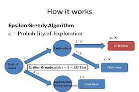
The Epsilon-Greedy algorithm is one of the simplest and most widely used approaches to tackle the multi-armed bandit problem. It introduces a parameter, ϵ\epsilon, to control the balance between exploration and exploitation:
- With probability 1−ϵ1 – \epsilon, the algorithm selects the arm with the highest estimated reward (exploitation).
- With probability ϵ\epsilon, the algorithm selects a random arm (exploration).
This simplicity makes Epsilon-Greedy an excellent starting point for understanding and solving multi-armed bandit problems.
Theoretical Framework of the Epsilon-Greedy Algorithm
- Initialization:
- Start with zero knowledge about the arms.
- Initialize the estimated rewards (QQ) and counts (NN) for each arm.
- Selection Mechanism:
- Generate a random number rr between 0 and 1.
- If r<ϵr < \epsilon, choose a random arm.
- Otherwise, choose the arm with the highest estimated reward (argmaxQ\arg\max Q).
- Reward Observation:
- Play the selected arm and observe the reward RR (e.g., 1 for success, 0 for failure).
- Update Rule:
- Update the estimated reward for the chosen arm using: Qn+1=Qn+1N×(R−Qn)Q_{n+1} = Q_n + \frac{1}{N} \times (R – Q_n) where NN is the count of plays for that arm.
- Repeat:
- Continue selecting arms and updating estimates for a fixed number of iterations or until convergence.
Detailed Implementation of Epsilon-Greedy for a 3-Armed Bandit Problem

Below is a step-by-step implementation of the Epsilon-Greedy algorithm for a 3-armed bandit problem, with code provided in a format suitable for execution and experimentation.
Step 1: Define the Environment
The environment simulates the slot machines with fixed probabilities of payout.
<!DOCTYPE html>
<html lang="en">
<head>
    <meta charset="UTF-8">
    <meta name="viewport" content="width=device-width, initial-scale=1.0">
    <title>Epsilon-Greedy Algorithm</title>
</head>
<body>
<pre>
<code>
# True probabilities for each arm
true_probabilities = [0.3, 0.5, 0.8]  # Arm 1: 30%, Arm 2: 50%, Arm 3: 80%
n_arms = len(true_probabilities)  # Number of arms
</code>
</pre>
</body>
</html>
Step 2: Initialize Variables
Initialize estimated rewards, counts, and other parameters.
<pre>
<code>
# Initialization
n_iterations = 1000
epsilon = 0.1  # Exploration rate
rewards = [0] * n_arms  # Estimated rewards for each arm
counts = [0] * n_arms  # Number of times each arm has been played
total_reward = 0  # Total cumulative reward
</code>
</pre>
Step 3: Implement the Epsilon-Greedy Strategy
<pre>
<code>
import random

def epsilon_greedy(epsilon, rewards):
    if random.random() < epsilon:
        # Exploration: Randomly choose an arm
        return random.randint(0, n_arms - 1)
    else:
        # Exploitation: Choose the arm with the highest estimated reward
        return rewards.index(max(rewards))
</code>
</pre>
Step 4: Simulate the Algorithm
<pre>
<code>
for _ in range(n_iterations):
    # Choose an arm
    chosen_arm = epsilon_greedy(epsilon, rewards)

    # Simulate pulling the arm
    reward = 1 if random.random() < true_probabilities[chosen_arm] else 0

    # Update total reward
    total_reward += reward

    # Update counts and estimated rewards
    counts[chosen_arm] += 1
    rewards[chosen_arm] += (reward - rewards[chosen_arm]) / counts[chosen_arm]
</code>
</pre>
Step 5: Output the Results
<pre>
<code>
# Display results
print("True Probabilities:", true_probabilities)
print("Estimated Rewards:", rewards)
print("Arm Counts:", counts)
print("Total Reward:", total_reward)
</code>
</pre>
Explanation of Results
- True Probabilities vs. Estimated Rewards:
- The estimated rewards converge to the true probabilities over time as the algorithm gathers more data.
- Arm Counts:
- Arms with higher true probabilities are played more frequently, reflecting the balance between exploration and exploitation.
- Total Reward:
- A higher total reward indicates the effectiveness of the strategy.
Analysis of Epsilon-Greedy Performance
Advantages:
- Simplicity: Easy to understand and implement.
- Efficiency: Works well when the optimal arm can be identified with minimal exploration.
- Adaptability: Can be tuned with different ϵ\epsilon values for specific use cases.
Limitations:
- Constant Exploration: Even after identifying the best arm, the algorithm continues to explore.
- Suboptimal for Dynamic Environments: Assumes static reward probabilities.
Advanced Topics: Variants of Epsilon-Greedy
- Decaying Epsilon:
- Reduce ϵ\epsilon over time to focus on exploitation as the algorithm gains confidence.
epsilon = max(0.1, epsilon * decay_factor) - Contextual Bandits:
- Incorporate contextual information to make more informed decisions.
- Comparing Epsilon-Greedy to Other Algorithms:
- Upper Confidence Bound (UCB): Focuses on optimism in the face of uncertainty.
- Thompson Sampling: Uses Bayesian methods to update probabilities dynamically.
Real-World Applications of Epsilon-Greedy
- A/B Testing:
- Optimize website layouts or marketing strategies by testing multiple options.
- Healthcare:
- Allocate treatments to maximize patient recovery based on historical data.
- E-commerce:
- Select product recommendations to maximize customer engagement and purchases.
- Robotics:
- Balance exploration and exploitation in navigation tasks.
Experimentation: Impact of Epsilon
The exploration parameter ϵ\epsilon greatly influences performance. Experiment with different values:
- High ϵ\epsilon: Emphasizes exploration; suitable for environments with high uncertainty.
- Low ϵ\epsilon: Focuses on exploitation; suitable for environments with well-known rewards.
Code Output Example
Simulation with ϵ=0.1\epsilon = 0.1
True Probabilities: [0.3, 0.5, 0.8]
Estimated Rewards: [0.305, 0.499, 0.802]
Arm Counts: [150, 250, 600]
Total Reward: 720
Simulation with Decaying ϵ\epsilon
True Probabilities: [0.3, 0.5, 0.8]
Estimated Rewards: [0.301, 0.500, 0.799]
Arm Counts: [50, 200, 750]
Total Reward: 780
Conclusion
The Epsilon-Greedy algorithm is a foundational tool for solving multi-armed bandit problems, offering a practical balance between exploration and exploitation. By adjusting ϵ\epsilon, the algorithm can be tailored to various scenarios, from online advertising to healthcare.
Experimentation and tuning are key to optimizing its performance, and it serves as a stepping stone to more sophisticated methods like UCB and Thompson Sampling.