Upper Confidence Bound (UCB) vs. Thompson Sampling
http://Upper Confidence Bound (UCB) vs. Thompson Sampling
Introduction
In decision-making scenarios like advertising campaigns, online recommendation systems, and clinical trials, the Multi-Armed Bandit (MAB) problem often arises. This problem involves a fundamental trade-off between exploration (trying out less-tested options to gather more information) and exploitation (leveraging the currently best-known option to maximize rewards).
Two widely recognized algorithms for tackling MAB problems are Upper Confidence Bound (UCB) and Thompson Sampling. Both aim to optimize cumulative rewards but differ significantly in their methodologies and underlying principles. In this guide, we will explore each algorithm in depth, compare their mechanics, and analyze their best use cases.
Understanding Multi-Armed Bandit (MAB) Problems
Imagine you’re at a casino with several slot machines (arms), each with a different probability of winning. You aim to maximize your winnings over time by determining which machine pays out the most.
Challenges include:
- Exploration: Testing underperforming machines to estimate their payout probabilities.
- Exploitation: Focusing on the machine with the highest known probability of payout to maximize returns.
UCB and Thompson Sampling are popular strategies to balance this trade-off effectively.
What is Upper Confidence Bound (UCB)?
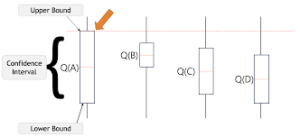
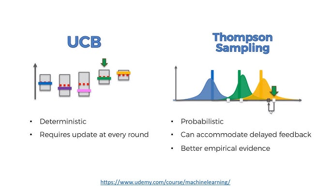
The Upper Confidence Bound (UCB) algorithm is based on the principle of optimism under uncertainty. It prioritizes actions with higher upper bounds on potential rewards. The key idea is to account for both the estimated reward (mean) and the uncertainty (variance) associated with each option.
Mathematics Behind UCB
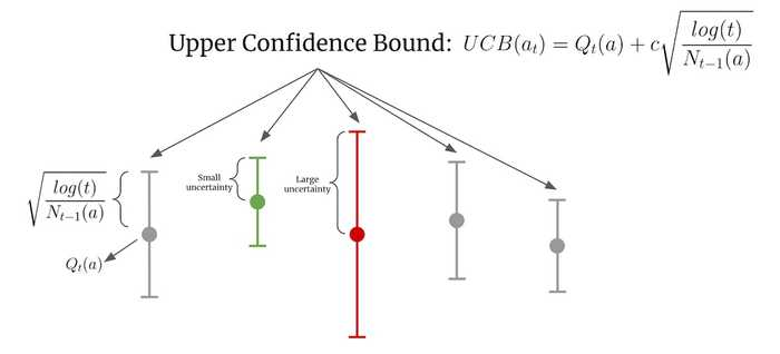
For each arm ii, the UCB value is calculated as: UCBi=μ^i+2ln(t)niUCB_i = \hat{\mu}_i + \sqrt{\frac{2 \ln(t)}{n_i}}
Where:
- μ^i\hat{\mu}_i: Empirical mean reward for arm ii.
- tt: Total number of rounds played.
- nin_i: Number of times arm ii has been pulled.
- 2ln(t)ni\sqrt{\frac{2 \ln(t)}{n_i}}: Exploration term to encourage pulling underexplored arms.
The algorithm selects the arm with the highest UCBiUCB_i value.
Key Characteristics of UCB
- Deterministic Approach: Decisions are entirely based on computed bounds.
- Confidence Intervals: Focuses on arms with high potential rewards and less certainty.
- Simplistic Design: Computationally inexpensive and easy to implement.
Strengths and Limitations of UCB
Strengths:
- Performs well in stationary reward distributions where the probability of success for each arm does not change over time.
- Computationally efficient due to the absence of sampling.
Limitations:
- Struggles in non-stationary environments, as it does not adapt to changing probabilities.
- Lacks stochasticity, which can be limiting in certain scenarios.
Implementation of UCB
Here’s a simple implementation using HTML with embedded JavaScript:
<!DOCTYPE html>
<html>
<head>
    <title>UCB Algorithm Simulation</title>
</head>
<body>
<h1>Upper Confidence Bound Algorithm</h1>
<pre>
<script>
function upperConfidenceBound(rewards, n_arms, total_rounds) {
    let arm_counts = Array(n_arms).fill(0);
    let arm_rewards = Array(n_arms).fill(0);
    let ucb_values = Array(n_arms).fill(0);

    for (let t = 1; t <= total_rounds; t++) {
        for (let arm = 0; arm < n_arms; arm++) {
            if (arm_counts[arm] === 0) {
                ucb_values[arm] = Infinity; // Pull each arm at least once
            } else {
                let avg_reward = arm_rewards[arm] / arm_counts[arm];
                ucb_values[arm] = avg_reward + Math.sqrt((2 * Math.log(t)) / arm_counts[arm]);
            }
        }

        let best_arm = ucb_values.indexOf(Math.max(...ucb_values));
        let reward = rewards[best_arm](); // Simulate pulling the arm
        arm_counts[best_arm]++;
        arm_rewards[best_arm] += reward;
    }

    return arm_rewards.map((r, i) => r / arm_counts[i]); // Return average rewards
}
</script>
</pre>
</body>
</html>
What is Thompson Sampling?
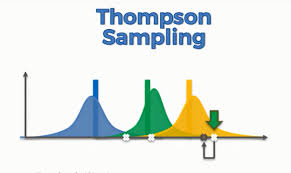
Thompson Sampling is a probabilistic algorithm rooted in Bayesian inference. It models the reward distribution of each arm and selects the arm based on posterior sampling. Unlike UCB, Thompson Sampling explicitly incorporates randomness into decision-making, which makes it highly adaptive.
Mathematics Behind Thompson Sampling
Thompson Sampling involves:
- Maintaining a prior distribution for each arm.
- Updating the prior using observed rewards to obtain a posterior distribution.
- Sampling from the posterior distribution for each arm.
- Selecting the arm with the highest sampled reward.
For binary rewards, the Beta distribution is commonly used:
- Prior: Beta(α,β)Beta(\alpha, \beta)
- Posterior update: After observing ss successes and ff failures: Beta(α+s,β+f)Beta(\alpha + s, \beta + f)
Key Characteristics of Thompson Sampling
- Stochastic Approach: Decisions involve randomness, leading to better exploration.
- Bayesian Foundation: Naturally balances exploration and exploitation using probability distributions.
- Flexibility: Adapts well to dynamic and non-stationary environments.
Strengths and Limitations of Thompson Sampling
Strengths:
- Performs well in dynamic reward environments where probabilities evolve over time.
- Efficiently balances exploration and exploitation through sampling.
Limitations:
- Computationally more intensive than UCB due to Bayesian updates.
- Requires knowledge of probability distributions.
Implementation of Thompson Sampling
Below is an HTML example using JavaScript:
<!DOCTYPE html>
<html>
<head>
    <title>Thompson Sampling Simulation</title>
</head>
<body>
<h1>Thompson Sampling Algorithm</h1>
<pre>
<script>
function thompsonSampling(rewards, n_arms, total_rounds) {
    let successes = Array(n_arms).fill(0);
    let failures = Array(n_arms).fill(0);

    for (let t = 0; t < total_rounds; t++) {
        let samples = Array(n_arms).fill(0);
        for (let arm = 0; arm < n_arms; arm++) {
            let alpha = 1 + successes[arm];
            let beta = 1 + failures[arm];
            samples[arm] = Math.random() * (alpha / (alpha + beta));
        }

        let best_arm = samples.indexOf(Math.max(...samples));
        let reward = rewards[best_arm](); // Simulate pulling the arm

        if (reward === 1) successes[best_arm]++;
        else failures[best_arm]++;
    }

    return successes.map((s, i) => s / (successes[i] + failures[i])); // Return probabilities
}
</script>
</pre>
</body>
</html>
Comparison Between UCB and Thompson Sampling
| Aspect | UCB | Thompson Sampling |
|---|---|---|
| Exploration | Explicit via confidence bounds | Implicit via posterior sampling |
| Exploitation | Deterministic | Stochastic |
| Computational Cost | Low | Medium (requires Bayesian updates) |
| Adaptability | Poor in non-stationary environments | High adaptability |
| Randomness | None | High |
| Ease of Use | Simple to implement | Requires understanding of Bayesian methods |
Best Use Cases
Upper Confidence Bound (UCB):
- Stationary Environments: Where the reward probabilities for each arm remain constant.
- Applications: Online advertisement testing, static A/B testing.
Thompson Sampling:
- Dynamic Environments: Where the reward probabilities evolve over time.
- Applications: Clinical trials, dynamic pricing, recommendation systems.
Conclusion
Both Upper Confidence Bound (UCB) and Thompson Sampling offer unique approaches to solving Multi-Armed Bandit problems. UCB is best suited for environments where simplicity and low computational costs are priorities. In contrast, Thompson Sampling thrives in more complex, dynamic scenarios due to its probabilistic nature.
Ultimately, the choice between the two depends on your specific problem requirements. For beginners, UCB provides an easier entry point, while those comfortable with Bayesian methods may prefer the flexibility of Thompson Sampling.
Which algorithm would you use for your next project? Let us know in the comments!