Key Components of a Markov Decision Process (MDP) and Real-World Applications
http://Key Components of a Markov Decision Process (MDP) and Real-World Applications
Introduction to Markov Decision Process (MDP)
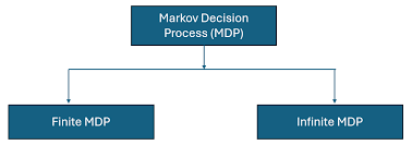
A Markov Decision Process (MDP) is a mathematical framework for modeling decision-making scenarios where the outcomes are influenced by both deterministic and stochastic elements. It is widely used in the fields of artificial intelligence, reinforcement learning, operations research, and economics to solve complex decision-making problems.
MDPs provide a structured way to make a sequence of decisions, considering the immediate rewards and future consequences of actions. This makes them particularly useful for systems where a series of choices leads to long-term outcomes, such as autonomous vehicles, game strategies, and resource optimization.
Key Components of an MDP
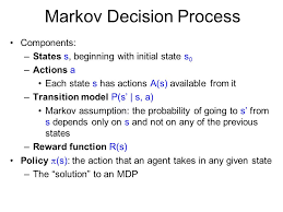
An MDP is formally represented by a tuple (S,A,T,R,γ)(S, A, T, R, \gamma), which includes the following components:
1. States (S):
- Definition: Represents all possible situations or configurations of the environment.
- Characteristics:
- States must encapsulate all relevant information needed for decision-making.
- The process is said to have the Markov property, meaning the future state depends only on the current state and action, not on past states.
- Example: In a warehouse robot, a state could include the robot’s location, its current load, and the surrounding obstacles.
2. Actions (A):
- Definition: A set of actions available to the agent at any given state.
- Characteristics:
- Actions determine how the agent interacts with the environment.
- Actions can vary depending on the state.
- Example: In a self-driving car, actions might include accelerating, braking, turning left, or turning right.
3. Transition Function (T):
- Definition: A probability function that defines the likelihood of moving to a new state s′s’ after taking action aa in state ss. Represented as T(s,a,s′)T(s, a, s’).
- Characteristics:
- Captures the uncertainty in the environment.
- Can be deterministic (always results in the same next state) or stochastic (results vary probabilistically).
- Example: In weather prediction, the transition function might define the probability of rain tomorrow given today’s conditions.
4. Rewards (R):
- Definition: The immediate numerical reward received after transitioning from state ss to s′s’ by taking action aa. Represented as R(s,a,s′)R(s, a, s’).
- Characteristics:
- Rewards are critical for defining the agent’s objectives.
- They can be positive (reward) or negative (penalty).
- Example: In a game, a player might receive points for defeating an opponent and lose points for failing a mission.
5. Policy (π\pi):
- Definition: A policy defines the strategy the agent uses to decide its actions at each state. It can be:
- Deterministic Policy (π(s)=a\pi(s) = a): Always selects the same action for a given state.
- Stochastic Policy (π(a∣s)\pi(a|s)): Specifies probabilities for selecting each action.
- Example: In a supply chain, the policy could decide the optimal number of products to stock based on current inventory.
6. Discount Factor (γ\gamma):
- Definition: A value between 0 and 1 that represents the importance of future rewards relative to immediate rewards.
- Characteristics:
- γ=0\gamma = 0: The agent is myopic and considers only immediate rewards.
- γ=1\gamma = 1: The agent is far-sighted and values future rewards equally with immediate rewards.
- Example: In investment strategies, a high discount factor reflects long-term financial planning.
Solving an MDP
The goal in solving an MDP is to find an optimal policy π∗\pi^* that maximizes the expected cumulative reward over time. There are two main approaches:
1. Value Iteration
This method computes the value of each state under an optimal policy by iteratively updating the state values based on the Bellman Equation: V(s)=maxa∑s′T(s,a,s′)[R(s,a,s′)+γV(s′)]V(s) = \max_a \sum_{s’} T(s, a, s’) \left[ R(s, a, s’) + \gamma V(s’) \right]
2. Policy Iteration
This method alternates between:
- Policy Evaluation: Compute the value function for a fixed policy.
- Policy Improvement: Update the policy to maximize the cumulative reward.
Real-World Application: Autonomous Vehicle Navigation

Problem Description:
An autonomous vehicle (AV) must navigate a city while optimizing for safety, speed, and fuel efficiency.
MDP Representation for the AV Problem
- States:
- Vehicle position, speed, traffic conditions, and nearby obstacles.
- Actions:
- Accelerate, decelerate, turn left, turn right, or maintain speed.
- Transition Function (T):
- Captures the probability of moving to a new state based on current speed, actions, and environmental conditions.
- Rewards:
- Positive rewards for reaching the destination quickly and safely.
- Negative rewards (penalties) for collisions, excessive braking, or violations.
- Policy:
- A policy defines how the AV reacts to traffic scenarios, e.g., slowing down when approaching a crowded intersection.
- Discount Factor (γ\gamma):
- A high discount factor ensures long-term goals (reaching the destination safely) are prioritized over immediate gains (speeding).
MDP Implementation for Navigation

Below is a Python implementation of a simplified grid-world problem for autonomous navigation:
<!DOCTYPE html>
<html>
<head>
    <title>MDP for Autonomous Navigation</title>
    <style>
        pre {
            background-color: #f4f4f4;
            padding: 10px;
            border-radius: 5px;
            overflow: auto;
        }
    </style>
</head>
<body>
    <h2>MDP Python Code for Autonomous Navigation</h2>
    <pre>
import numpy as np

# Define the grid world
grid_size = (5, 5)
actions = ["up", "down", "left", "right"]

# Rewards and transitions
rewards = np.zeros(grid_size)
rewards[4, 4] = 10  # Goal state reward

# Define transition probabilities
def get_next_state(state, action):
    x, y = state
    if action == "up" and x > 0:
        return (x - 1, y)
    elif action == "down" and x < grid_size[0] - 1:
        return (x + 1, y)
    elif action == "left" and y > 0:
        return (x, y - 1)
    elif action == "right" and y < grid_size[1] - 1:
        return (x, y + 1)
    return state  # No movement if action invalid

# Value iteration
values = np.zeros(grid_size)
gamma = 0.9  # Discount factor

for _ in range(100):
    new_values = values.copy()
    for x in range(grid_size[0]):
        for y in range(grid_size[1]):
            state = (x, y)
            action_values = []
            for action in actions:
                next_state = get_next_state(state, action)
                reward = rewards[next_state]
                action_values.append(reward + gamma * values[next_state])
            new_values[state] = max(action_values)
    values = new_values

print("Optimal State Values:")
print(values)
    </pre>
</body>
</html>
Interpretation of Results
- The grid values represent the expected cumulative reward from each state.
- The optimal path for the AV can be derived by following the highest-value states.
Other Real-World Applications of MDPs
- Healthcare:
- Application: Personalized treatment plans.
- MDP Role: Balances the immediate effects of medication with long-term health outcomes.
- Finance:
- Application: Portfolio optimization.
- MDP Role: Helps investors decide on asset allocations to maximize returns while minimizing risks.
- Robotics:
- Application: Path planning for robotic arms.
- MDP Role: Ensures optimal movements while avoiding collisions.
- Customer Service:
- Application: AI chatbots for dynamic responses.
- MDP Role: Determines the best response based on user queries and history.
- Energy Management:
- Application: Smart grid optimization.
- MDP Role: Balances energy generation, storage, and distribution efficiently.
Conclusion
Markov Decision Processes offer a versatile framework for solving decision-making problems in uncertain environments. By modeling real-world scenarios with states, actions, transitions, rewards, and policies, MDPs enable the design of intelligent systems that maximize cumulative benefits.
For practical exploration, the Python implementation provided can be expanded for more complex problems. From self-driving cars to healthcare, MDPs are at the core of many transformative applications, driving innovation and efficiency across industries.