The Bellman Equation for Value Iteration: A Detailed Exploration 2024

http://The Bellman Equation for Value Iteration

The Bellman Equation for Value Iteration

Markov Decision Processes (MDPs) provide a robust mathematical framework for modeling decision-making in scenarios where outcomes are partly random and partly under an agent’s control. The Bellman Equation is a cornerstone of solving MDPs, playing a central role in reinforcement learning and dynamic programming. It facilitates efficient computation of optimal strategies through methods like value iteration and policy iteration.

This blog delves deep into the Bellman Equation, its role in solving MDPs, and how value iteration leverages it for finding optimal policies.

Introduction to Markov Decision Processes (MDPs)

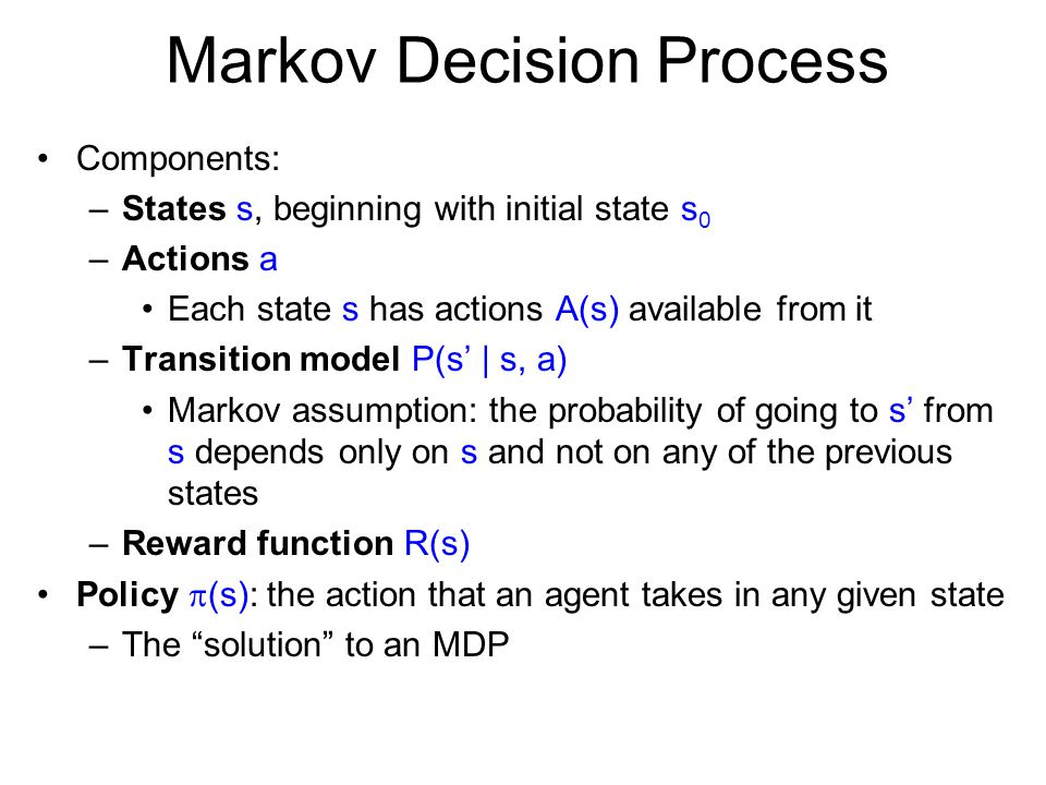
An MDP is defined by the following components:

States (SS): The set of all possible states an agent can occupy.
Actions (AA): The set of actions the agent can take.
Transition Probabilities (P(s′∣s,a)P(s’|s, a)): The probability of moving to state s′s’ when action aa is taken in state ss.
Rewards (R(s,a,s′)R(s, a, s’)): The reward received for transitioning from state ss to s′s’ by taking action aa.
Discount Factor (γ\gamma): A factor 0≤γ≤10 \leq \gamma \leq 1 that determines the importance of future rewards compared to immediate ones.

Objective of Solving MDPs

The goal is to find an optimal policy π∗\pi^* that maximizes the expected cumulative reward over time. A policy π(a∣s)\pi(a|s) specifies the probability of taking action aa in state ss.

The Value Function and its Importance

The value function quantifies the long-term value of a state under a given policy. For a policy π\pi, the value function Vπ(s)V^{\pi}(s) is: Vπ(s)=E[∑t=0∞γtR(st,at,st+1)∣s0=s,π]V^{\pi}(s) = \mathbb{E}\left[ \sum_{t=0}^{\infty} \gamma^t R(s_t, a_t, s_{t+1}) \mid s_0 = s, \pi \right]

Here:

R(st,at,st+1)R(s_t, a_t, s_{t+1}): Reward at time tt for taking action ata_t in state sts_t.
γt\gamma^t: Discounted weight of future rewards.

The value function provides:

A measure of the quality of a state.
A mechanism to compare different policies.

The Bellman Equation

The Bellman Equation breaks down the value function recursively. For a given policy π\pi: Vπ(s)=∑a∈Aπ(a∣s)∑s′∈SP(s′∣s,a)[R(s,a,s′)+γVπ(s′)]V^{\pi}(s) = \sum_{a \in A} \pi(a|s) \sum_{s’ \in S} P(s’|s, a) \left[ R(s, a, s’) + \gamma V^{\pi}(s’) \right]

Explanation of Components

π(a∣s)\pi(a|s): The likelihood of taking action aa in state ss under policy π\pi.
P(s′∣s,a)P(s’|s, a): Transition probability of reaching state s′s’ from ss using action aa.
R(s,a,s′)R(s, a, s’): Immediate reward for the transition.
γVπ(s′)\gamma V^{\pi}(s’): Discounted future reward from successor state s′s’.

This equation represents the expected value of a state as a function of immediate rewards and the expected value of future states.

Bellman Optimality Equation

For the optimal policy π∗\pi^*, the Bellman Optimality Equation is: V∗(s)=max⁡a∈A∑s′∈SP(s′∣s,a)[R(s,a,s′)+γV∗(s′)]V^*(s) = \max_{a \in A} \sum_{s’ \in S} P(s’|s, a) \left[ R(s, a, s’) + \gamma V^*(s’) \right]

This equation asserts that the value of a state under the optimal policy is the maximum expected value obtainable by taking the best possible action.

Value Iteration: Solving MDPs Using the Bellman Equation

What is Value Iteration?

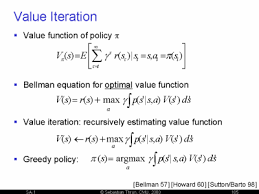
Value iteration is an iterative algorithm that computes the optimal value function V∗(s)V^*(s) by repeatedly applying the Bellman Optimality Equation until convergence. Once V∗(s)V^*(s) is computed, the optimal policy π∗\pi^* can be derived.

Steps in Value Iteration

Initialization: Set V(s)=0V(s) = 0 (or arbitrary values) for all states.
Value Update: For each state ss, update V(s)V(s) using: V(s)←max⁡a∈A∑s′∈SP(s′∣s,a)[R(s,a,s′)+γV(s′)]V(s) \gets \max_{a \in A} \sum_{s’ \in S} P(s’|s, a) \left[ R(s, a, s’) + \gamma V(s’) \right]
Convergence Check: Stop when the value function changes by less than a small threshold (ϵ\epsilon) for all states.
Policy Extraction: Derive the optimal policy: π∗(s)=arg⁡max⁡a∈A∑s′∈SP(s′∣s,a)[R(s,a,s′)+γV(s′)]\pi^*(s) = \arg\max_{a \in A} \sum_{s’ \in S} P(s’|s, a) \left[ R(s, a, s’) + \gamma V(s’) \right]

Pseudo-code for Value Iteration

<!DOCTYPE html>
<html>
<head>
    <title>Value Iteration Algorithm</title>
</head>
<body>
    <pre>
function ValueIteration(states, actions, P, R, gamma, threshold):
    Initialize V[s] = 0 for all states s
    repeat:
        Delta = 0
        for each state s:
            v = V[s]
            V[s] = max_a sum_{s'} P(s'|s, a) * (R(s, a, s') + gamma * V[s'])
            Delta = max(Delta, abs(v - V[s]))
        if Delta < threshold:
            break
    policy = {}
    for each state s:
        policy[s] = argmax_a sum_{s'} P(s'|s, a) * (R(s, a, s') + gamma * V[s'])
    return V, policy
    </pre>
</body>
</html>

Convergence of Value Iteration

Value iteration converges because the Bellman Equation is a contraction mapping. The value updates bring the value function closer to the true optimal values V∗V^* in each iteration.

Example: Grid World

Let’s consider a simple grid world with the following properties:

States (SS): Cells in a 3×3 grid.
Actions (AA): {Up, Down, Left, Right}.
Rewards (RR): -1 for each step, +10 for reaching the goal.
Transitions (PP): Deterministic (action always succeeds).

Python Code for Value Iteration

<!DOCTYPE html>
<html>
<head>
    <title>Value Iteration in Grid World</title>
</head>
<body>
    <pre>
import numpy as np

# Define MDP components
grid_size = 3
actions = ["up", "down", "left", "right"]
gamma = 0.9  # Discount factor
reward = -1  # Step penalty
goal = (2, 2)

# Transition function
def get_transitions(state, action):
    x, y = state
    if state == goal:
        return [(1.0, state, 0)]
    if action == "up":
        new_state = (max(x - 1, 0), y)
    elif action == "down":
        new_state = (min(x + 1, grid_size - 1), y)
    elif action == "left":
        new_state = (x, max(y - 1, 0))
    elif action == "right":
        new_state = (x, min(y + 1, grid_size - 1))
    return [(1.0, new_state, reward)]

# Value iteration
def value_iteration(threshold=1e-6):
    V = np.zeros((grid_size, grid_size))
    while True:
        delta = 0
        new_V = V.copy()
        for x in range(grid_size):
            for y in range(grid_size):
                state = (x, y)
                values = []
                for action in actions:
                    transitions = get_transitions(state, action)
                    value = sum(prob * (r + gamma * V[s[0], s[1]]) for prob, s, r in transitions)
                    values.append(value)
                new_V[x, y] = max(values)
                delta = max(delta, abs(new_V[x, y] - V[x, y]))
        V = new_V
        if delta < threshold:
            break
    return V

optimal_values = value_iteration()
print(optimal_values)

Applications of the Bellman Equation

Robotics: Optimizing robot movement in uncertain environments.
Game Theory: Computing strategies in stochastic games.
Operations Research: Resource allocation problems.
Finance: Portfolio optimization and pricing options.

Conclusion

The Bellman Equation is central to solving MDPs because it provides a recursive structure to compute value functions. Through algorithms like value iteration, it helps derive optimal policies that maximize long-term rewards. Understanding this concept is crucial for fields like reinforcement learning, robotics, and AI planning.

This exploration should give you the depth and clarity needed to appreciate the Bellman Equation’s significance in modern computational problems.