Deterministic vs. Stochastic Policies in Markov Decision Processes (MDPs)
http://Deterministic vs. Stochastic Policies in Markov Decision Processes (MDPs)
Markov Decision Processes (MDPs) provide a mathematical framework for modeling decision-making situations where outcomes are partly under the control of a decision-maker and partly influenced by chance. At the heart of solving MDPs is the concept of a policy, which dictates the actions an agent should take in various states to maximize rewards over time. In this blog, we explore the difference between deterministic policies and stochastic policies, their roles in MDPs, and scenarios where one may be preferred over the other.
What is a Policy in MDP?
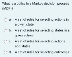
A policy in the context of an MDP defines a strategy or rule that an agent follows to choose actions based on the current state. Formally, a policy is a mapping from states (SS) to actions (AA): π(s)→a\pi(s) \rightarrow a
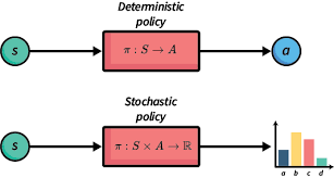
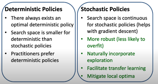
- Deterministic Policy: Maps each state to a specific action deterministically.
- Stochastic Policy: Maps each state to a probability distribution over actions.
Deterministic Policies
Definition
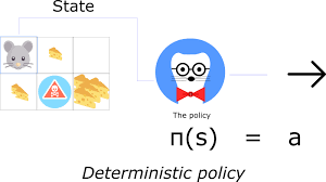
A deterministic policy specifies a single action to be taken in a given state. Mathematically: π(s)=a\pi(s) = a
Here, aa is a specific action determined with certainty.
Characteristics
- Simplicity: Easy to implement and computationally less demanding.
- Reproducibility: Guarantees the same outcome for a given state every time.
- Optimality: For many problems with finite state and action spaces, a deterministic policy suffices to achieve optimality.
Example
In a navigation problem, if an agent is in a specific grid cell, a deterministic policy might always dictate moving north if there is a reward in that direction.
Stochastic Policies
Definition
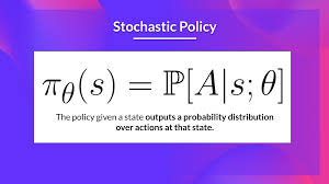
A stochastic policy defines a probability distribution over actions for each state. Mathematically: π(a∣s)=P(A=a∣S=s)\pi(a | s) = P(A = a | S = s)
Here, P(A=a∣S=s)P(A = a | S = s) represents the probability of taking action aa when in state ss.
Characteristics
- Flexibility: Allows exploration of multiple actions, which can be beneficial in non-deterministic or noisy environments.
- Adaptability: Suitable for scenarios with uncertainty or partial observability.
- Optimality in Complex Scenarios: Some problems (e.g., adversarial games) may require stochastic policies for optimal behavior.
Example
In a game of poker, a stochastic policy might assign probabilities to bluffing or folding based on the current state of the game.
Comparison: Deterministic vs. Stochastic Policies
Key Differences
| Feature | Deterministic Policy | Stochastic Policy |
|---|---|---|
| Definition | Maps states to single actions | Maps states to probability distributions over actions |
| Exploration | Limited to pre-determined paths | Encourages exploration of multiple actions |
| Optimality | Optimal in simple MDPs | Optimal in environments with uncertainty or noise |
| Complexity | Simpler to compute | Computationally more demanding due to probability distributions |
| Robustness | Less robust in noisy environments | More robust to uncertainties and stochastic dynamics |
Applications
When to Use Deterministic Policies
- Static Environments: Where transitions and rewards are deterministic.
- Low Noise: When the environment is predictable.
- Optimization Focus: Problems where simplicity and speed are prioritized.
When to Use Stochastic Policies
- Dynamic Environments: Where outcomes of actions are uncertain.
- Exploration Needs: Problems requiring exploration of multiple strategies.
- Game Theory: Scenarios involving adversarial agents or mixed strategies.
Mathematical Formulation in MDPs
Bellman Equation with Deterministic Policies
For a deterministic policy π\pi, the Bellman equation can be written as: Vπ(s)=R(s,π(s))+γ∑s′P(s′∣s,π(s))Vπ(s′)V^\pi(s) = R(s, \pi(s)) + \gamma \sum_{s’} P(s’|s, \pi(s)) V^\pi(s’)
Here:
- Vπ(s)V^\pi(s) is the value of state ss under policy π\pi.
- R(s,π(s))R(s, \pi(s)) is the reward received by taking action π(s)\pi(s).
- P(s′∣s,π(s))P(s’|s, \pi(s)) is the transition probability to state s′s’.
- γ\gamma is the discount factor.
Bellman Equation with Stochastic Policies
For a stochastic policy π(a∣s)\pi(a|s), the Bellman equation generalizes to: Vπ(s)=∑aπ(a∣s)[R(s,a)+γ∑s′P(s′∣s,a)Vπ(s′)]V^\pi(s) = \sum_{a} \pi(a|s) \left[ R(s, a) + \gamma \sum_{s’} P(s’|s, a) V^\pi(s’) \right]
Here:
- The value Vπ(s)V^\pi(s) depends on the expected value of rewards, taking into account the probability distribution over actions.
Example with Code: Deterministic vs. Stochastic Policies
Problem: Grid Navigation
Consider a grid world where an agent moves to maximize rewards. The states are grid cells, and actions are {Up, Down, Left, Right}.
Deterministic Policy
<pre>
<code>
# Deterministic Policy Implementation
states = ["A", "B", "C", "D"]
actions = ["Up", "Down", "Left", "Right"]
policy = {
    "A": "Up",
    "B": "Right",
    "C": "Down",
    "D": "Left"
}

def deterministic_policy(state):
    return policy[state]

# Test the deterministic policy
current_state = "A"
print(f"Action for state {current_state}: {deterministic_policy(current_state)}")
</code>
</pre>
Stochastic Policy
<pre>
<code>
# Stochastic Policy Implementation
import random

states = ["A", "B", "C", "D"]
actions = ["Up", "Down", "Left", "Right"]
policy = {
    "A": {"Up": 0.7, "Right": 0.3},
    "B": {"Right": 1.0},
    "C": {"Down": 0.5, "Left": 0.5},
    "D": {"Left": 0.8, "Up": 0.2}
}

def stochastic_policy(state):
    action_probs = policy[state]
    actions, probabilities = zip(*action_probs.items())
    return random.choices(actions, probabilities)[0]

# Test the stochastic policy
current_state = "A"
print(f"Action for state {current_state}: {stochastic_policy(current_state)}")
</code>
</pre>
Advantages and Limitations
Deterministic Policies
Advantages:
- Easy to understand and implement.
- Computationally efficient.
- Sufficient for many simple MDPs.
Limitations:
- Limited exploration capability.
- Vulnerable to suboptimality in noisy environments.
Stochastic Policies
Advantages:
- Encourages exploration and adaptability.
- Handles uncertainty better.
- Essential in adversarial or mixed-strategy environments.
Limitations:
- More complex to compute.
- May require significant computational resources.
Conclusion
Understanding the distinction between deterministic and stochastic policies is crucial for solving MDPs effectively. While deterministic policies are optimal for many simple problems, stochastic policies provide the flexibility and robustness required in complex, uncertain, or adversarial environments.
By balancing simplicity and adaptability, you can choose the right policy type for your specific application, whether it involves robotics, game theory, or reinforcement learning systems.
This blog highlighted key concepts, mathematical formulations, examples, and the trade-offs between deterministic and stochastic policies in MDPs. If you’d like to explore more, stay tuned for our upcoming articles on advanced reinforcement learning topics!