Understanding Rewards and Returns in Markov Decision Processes (MDPs)
http://Understanding Rewards and Returns in Markov Decision Processes (MDPs)
Markov Decision Processes (MDPs) are the cornerstone of reinforcement learning, a branch of machine learning that deals with decision-making in environments where outcomes are uncertain and delayed. MDPs provide a mathematical framework for modeling sequential decision-making problems, where an agent interacts with an environment to achieve some goal, typically by maximizing cumulative rewards over time. To fully grasp how an agent learns and makes decisions in an MDP, it’s essential to understand the concepts of rewards and returns and how they are computed. Additionally, the concept of the expected return is central to evaluating policies and guiding the agent’s learning process. In this blog, we’ll explore these concepts in depth, explaining how they are computed, why they are important, and how they help agents make optimal decisions.
What is an MDP?
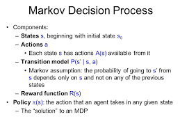
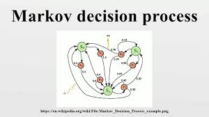
An MDP is defined by a tuple (S,A,P,R,γ)(S, A, P, R, \gamma), where:
- S: A set of states representing all possible situations the agent could be in.
- A: A set of actions the agent can take in each state.
- P: A state transition probability function, where P(s′∣s,a)P(s’|s, a) represents the probability of transitioning to state s′s’ after taking action aa in state ss.
- R: A reward function R(s,a,s′)R(s, a, s’) that gives the immediate reward the agent receives after transitioning from state ss to state s′s’ by taking action aa.
- γ\gamma: A discount factor, 0≤γ≤10 \leq \gamma \leq 1, that controls how much the agent values future rewards relative to immediate rewards. A discount factor close to 1 means the agent values future rewards almost as much as the present ones.
States, Actions, and Rewards
- States (S): The set of states SS represents all the possible configurations or situations of the environment that the agent might encounter. For example, in a robotic navigation task, the state could represent the robot’s position in a grid, while in a game, it could represent the game board configuration.
- Actions (A): The set of actions AA represents the possible moves or decisions the agent can make in any given state. The agent’s goal is to choose the right actions to maximize its rewards. For instance, in the grid navigation task, actions could be “move up”, “move down”, “move left”, and “move right”.
- Rewards (R): The reward function R(s,a,s′)R(s, a, s’) provides immediate feedback to the agent after each action. It tells the agent how good or bad its decision was in terms of achieving the goal. In some cases, the reward might be a positive value for a successful action (like reaching a goal) or a negative value (like hitting an obstacle). In reinforcement learning, the goal of the agent is to maximize the cumulative reward over time.
Computing Rewards and Returns
At each step in an MDP, the agent performs an action aa in state ss, and the environment responds with a new state s′s’ and a reward R(s,a,s′)R(s, a, s’). The agent’s ultimate objective is to maximize the cumulative reward it receives over time, but rewards are often delayed. For instance, in a game, the agent may receive a reward only after completing a sequence of actions. This delay creates the challenge of determining which actions in the past contributed to the eventual success or failure.
Immediate Reward
The immediate reward RtR_t is the feedback the agent receives for taking an action at time step tt. This reward is used to inform the agent about the effectiveness of its actions, but alone, it doesn’t give enough information about long-term success. The agent needs to evaluate how current actions impact future rewards, which leads to the concept of returns.
The Return: What Is It and How Is It Computed?
In reinforcement learning, returns refer to the total accumulated rewards an agent receives over time. Since the agent’s decisions at each step can influence future rewards, returns account for the long-term consequences of those decisions. A return is computed as the sum of rewards over a period of time, typically discounted to account for the fact that future rewards are less certain and often less valuable than immediate ones.
Finite Horizon Return
In problems with a finite time horizon (i.e., the agent’s interaction with the environment is limited to a specific number of steps), the return is simply the sum of the rewards from the current time step until the end of the episode. Mathematically, the return GtG_t at time step tt is: Gt=Rt+Rt+1+⋯+RTG_t = R_t + R_{t+1} + \dots + R_T
where TT is the final time step of the episode. The agent’s goal is to maximize this return over the course of the episode.
Infinite Horizon Return
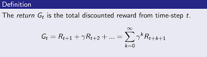
In many reinforcement learning problems, the agent operates indefinitely, and there is no fixed endpoint. To handle such problems, we compute the discounted return over an infinite horizon. The discounted return allows the agent to weigh future rewards less than immediate ones, preventing the sum from becoming infinite.
The discounted return GtG_t at time step tt is: Gt=Rt+γRt+1+γ2Rt+2+…G_t = R_t + \gamma R_{t+1} + \gamma^2 R_{t+2} + \dots
where γ\gamma is the discount factor, a number between 0 and 1. A higher value of γ\gamma means the agent values future rewards more, while a lower value of γ\gamma makes the agent focus more on immediate rewards.
The discounted return ensures that the value of the return remains finite even when the agent interacts with the environment indefinitely.
Why Discounted Return?
The discount factor γ\gamma is essential for several reasons:
- Uncertainty of Future Rewards: Future rewards are less certain because the agent’s future decisions and the environment’s reactions are not predictable. Discounting reduces the influence of distant future rewards.
- Prioritizing Immediate Rewards: In many scenarios, immediate rewards are more tangible and relevant than rewards received far in the future. Discounting allows the agent to prioritize short-term gains over long-term rewards.
- Computational Stability: Without discounting, the value function might grow unboundedly, making it difficult to optimize policies effectively. The discount factor ensures that the return converges and remains manageable.
Expected Return: Why Is It So Important?
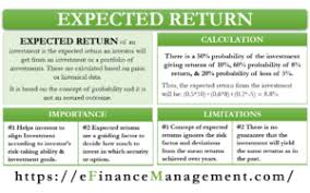
The expected return is a central concept in reinforcement learning. Since the agent doesn’t have perfect knowledge of the environment, it must make decisions based on the expected outcomes of its actions. The expected return gives the agent a way to evaluate how good a particular state or action is, based on the average outcomes it can expect, given the current policy.
Policy: A Strategy for Action
A policy π\pi is a mapping from states to actions, which defines the agent’s behavior in each state. A policy can be either:
- Deterministic: A fixed action is taken for each state, i.e., π(s)=a\pi(s) = a.
- Stochastic: A probability distribution over actions is defined for each state, i.e., π(a∣s)\pi(a|s) gives the probability of taking action aa when in state ss.
Value Functions and Expected Return
The value function Vπ(s)V^\pi(s) of a policy π\pi represents the expected return an agent can achieve starting from state ss and following policy π\pi. Mathematically, the value function is: Vπ(s)=E[Gt∣st=s,π]V^\pi(s) = \mathbb{E}\left[G_t | s_t = s, \pi\right]
where GtG_t is the return at time step tt, and the expectation is taken over all possible state-action sequences that might occur from state ss onwards, under policy π\pi.
For a state-action pair (s,a)(s, a), the Q-value Qπ(s,a)Q^\pi(s, a) represents the expected return when taking action aa in state ss, and then following the policy π\pi. The Q-value is given by: Qπ(s,a)=E[Gt∣st=s,at=a,π]Q^\pi(s, a) = \mathbb{E}\left[G_t | s_t = s, a_t = a, \pi \right]
Bellman Equations: Relationship Between Value Functions
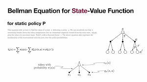
The Bellman equation provides a recursive relationship between the value of a state and the value of its successor states. For a given policy π\pi, the value function Vπ(s)V^\pi(s) satisfies the following equation: Vπ(s)=∑a∈Aπ(a∣s)∑s′∈SP(s′∣s,a)[R(s,a,s′)+γVπ(s′)]V^\pi(s) = \sum_{a \in A} \pi(a|s) \sum_{s’ \in S} P(s’|s, a) \left[ R(s, a, s’) + \gamma V^\pi(s’) \right]
Similarly, for the Q-value function: Qπ(s,a)=∑s′∈SP(s′∣s,a)[R(s,a,s′)+γ∑a′∈Aπ(a′∣s′)Qπ(s′,a′)]Q^\pi(s, a) = \sum_{s’ \in S} P(s’|s, a) \left[ R(s, a, s’) + \gamma \sum_{a’ \in A} \pi(a’|s’) Q^\pi(s’, a’) \right]
These equations are crucial for both evaluating and improving policies.
By iteratively solving the Bellman equations, we can find the optimal policy that maximizes the expected return.
Practical Example: Computing the Expected Return in Python
Let’s demonstrate how to compute the expected return in a simple environment using Monte Carlo methods. This method estimates the expected return by simulating episodes and averaging the returns.
import numpy as np

# Simple environment with two states (0 and 1)
class SimpleEnv:
    def __init__(self):
        self.state_space = [0, 1]
        self.action_space = [0, 1]
        self.state = 0

    def reset(self):
        self.state = 0
        return self.state

    def step(self, action):
        if self.state == 0:
            if action == 0:
                return 0, 0, True, {}  # No reward, done
            else:
                return 1, 1, False, {}  # Reward, not done
        else:
            return 1, 0, True, {}  # No reward, done

# Function to simulate an episode and compute the return
def simulate_episode(env, policy, gamma=0.9):
    episode = []
    state = env.reset()
    done = False

    while not done:
        action = policy[state]
        next_state, reward, done, _ = env.step(action)
        episode.append((state, action, reward, next_state))
        state = next_state

    return compute_return(episode, gamma)

# Function to compute the return from a list of (state, action, reward, next_state) tuples
def compute_return(episode, gamma):
    returns = []
    G = 0  # Initialize the return
    for state, action, reward, _ in reversed(episode):
        G = reward + gamma * G
        returns.insert(0, G)
    return returns

# Define a policy: action 1 in state 0, action 0 in state 1
policy = {0: 1, 1: 0}

# Simulate an episode and compute the return
env = SimpleEnv()
episode = simulate_episode(env, policy)
print("Episode returns:", episode)
In this code, we define a simple environment with two states and two actions. The policy is deterministic: take action 1 in state 0 and action 0 in state 1. We then simulate an episode and compute the return using the discount factor γ\gamma.
Conclusion
In Markov Decision Processes (MDPs), rewards, returns, and expected returns form the foundation for an agent’s decision-making process. Rewards are the immediate feedback that guide the agent’s actions, while returns provide a way to accumulate these rewards over time, considering both immediate and future outcomes. The expected return, which accounts for uncertainty and delayed consequences, is crucial for evaluating policies and guiding the agent towards optimal decision-making.
By understanding the mathematical underpinnings of rewards and returns, as well as the importance of discounting and the expected return, you can effectively design reinforcement learning algorithms that help agents learn optimal policies in complex, uncertain environments. Whether you’re building a simple navigation robot or designing a sophisticated game AI, these concepts are vital to the success of any reinforcement learning application.