The Role of State-Value and Action-Value Functions in Reinforcement Learning

http://The Role of State-Value and Action-Value Functions in Reinforcement Learning 2024

Reinforcement Learning (RL) is a branch of machine learning where agents learn to make decisions by interacting with an environment. The key idea is that an agent can take actions in an environment, receive feedback in the form of rewards, and use that feedback to learn how to make better decisions over time. One of the core aspects of RL is how the agent evaluates different states and actions in the environment. This evaluation is done using state-value functions and action-value functions, which are crucial to the decision-making process. In this blog, we will dive into the roles of these functions, how they influence an agent’s behavior, and their importance in reinforcement learning algorithms.

---

What Are State-Value and Action-Value Functions?

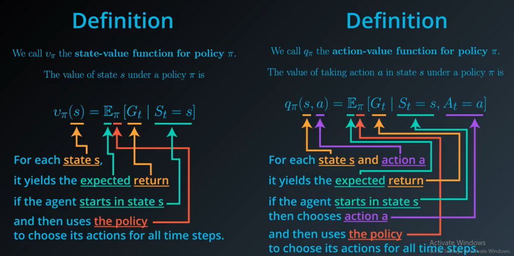
State-Value Function (V(s)V(s))

The state-value function is a measure of the long-term expected return (or cumulative reward) the agent can expect to receive starting from a particular state and following a specific policy. It is denoted as Vπ(s)V^\pi(s), where:

• ss represents a state in the environment.
• π\pi represents the policy, which is the strategy or rule that tells the agent which action to take in each state.

The state-value function gives a quantitative measure of how “good” it is to be in a given state under a specific policy. If an agent is in state ss, the state-value function Vπ(s)V^\pi(s) represents the expected return from that state onward, assuming the agent follows policy π\pi.

Mathematically, the state-value function is defined as: Vπ(s)=E[Gt∣st=s,π]V^\pi(s) = \mathbb{E}\left[G_t | s_t = s, \pi\right]

Where GtG_t is the return (the sum of discounted rewards) from time step tt onward, and the expectation is taken over all possible sequences of states and actions under the policy π\pi.

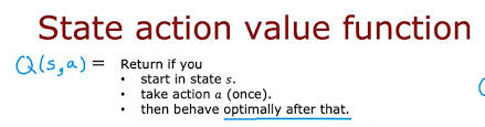
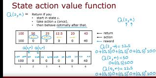
Action-Value Function (Q(s,a)Q(s, a))

The action-value function is similar to the state-value function, but it also considers the action the agent takes in a given state. It is denoted as Qπ(s,a)Q^\pi(s, a), where:

• ss represents a state.
• aa represents an action the agent can take in that state.
• π\pi represents the policy, which dictates how the agent behaves.

The action-value function Qπ(s,a)Q^\pi(s, a) gives the expected return when the agent starts from state ss, takes action aa, and then follows the policy π\pi. This means the action-value function helps evaluate the quality of taking a specific action in a given state, under a particular policy.

Mathematically, the action-value function is defined as: Qπ(s,a)=E[Gt∣st=s,at=a,π]Q^\pi(s, a) = \mathbb{E}\left[G_t | s_t = s, a_t = a, \pi\right]

Where, like in the state-value function, the expectation is over the possible outcomes of taking action aa in state ss and following policy π\pi.

---

How Do State-Value and Action-Value Functions Influence an Agent’s Decision-Making?

Both the state-value and action-value functions play critical roles in guiding an agent’s decisions, and they are fundamental to many reinforcement learning algorithms. Let’s explore how these functions influence decision-making and help the agent learn optimal behavior.

1. State-Value Function and Decision-Making

The state-value function is used to estimate the long-term benefit of being in a specific state. In an RL task, the agent’s goal is often to reach states with the highest possible value. Therefore, an agent can make decisions based on which state leads to the most favorable outcomes, according to the state-value function.

For example, in a grid world environment, the agent might want to move towards states with high Vπ(s)V^\pi(s) values because these states are more likely to lead to better rewards in the long run. However, since the agent cannot always directly choose the optimal state, it may need to evaluate each state’s value and act accordingly. The state-value function essentially provides a global view of which states are more desirable.

Influence on Policy:

• If the agent follows a greedy policy, it will always choose the action that leads to the highest-valued state, thus optimizing its decisions for long-term success.
• If the agent is using an exploratory policy (e.g., epsilon-greedy), it will still be guided by the state values but will occasionally explore other actions.

2. Action-Value Function and Decision-Making

While the state-value function provides an evaluation of states, the action-value function takes it a step further by evaluating actions in addition to states. The action-value function is particularly useful when an agent needs to decide which action to take in a specific state to maximize long-term rewards.

For example, in a self-driving car, the action-value function helps the car decide whether to accelerate, brake, or turn at an intersection based on the expected future rewards for each action. It evaluates each action’s immediate reward as well as the future rewards that each action can lead to, guiding the agent to the most beneficial decision.

Influence on Policy:

• Greedy Policy: The agent will choose the action aa that maximizes Q(s,a)Q(s, a) for any state ss, as this will lead to the highest return.
• Exploration vs. Exploitation: If the agent is balancing exploration and exploitation, it might sometimes take actions that don’t maximize Q(s,a)Q(s, a) immediately but might reveal new and valuable information for future decisions.

---

Algorithms Using State-Value and Action-Value Functions

Many popular reinforcement learning algorithms, including Q-learning, SARSA, and Monte Carlo methods, rely on state-value and action-value functions to guide the agent’s learning process. These algorithms use the functions to estimate the long-term returns and improve the agent’s policy over time.

Q-learning

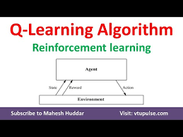
Q-learning is an off-policy algorithm that uses the action-value function Q(s,a)Q(s, a) to learn the optimal policy. The agent starts by exploring the environment and updating its action-value function iteratively based on the rewards it receives. The update rule for Q-learning is: Q(st,at)←Q(st,at)+α[Rt+1+γmax⁡a′Q(st+1,a′)−Q(st,at)]Q(s_t, a_t) \leftarrow Q(s_t, a_t) + \alpha \left[ R_{t+1} + \gamma \max_{a’} Q(s_{t+1}, a’) – Q(s_t, a_t) \right]

Where:

• α\alpha is the learning rate.
• γ\gamma is the discount factor.
• Rt+1R_{t+1} is the immediate reward.
• max⁡a′Q(st+1,a′)\max_{a’} Q(s_{t+1}, a’) is the maximum action-value for the next state.

Q-learning aims to find the optimal action-value function Q∗(s,a)Q^*(s, a) by continually updating the estimates. The agent will eventually converge to an optimal policy that maximizes the expected return, by always taking the action that maximizes the action-value.

SARSA

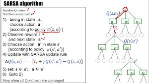
SARSA (State-Action-Reward-State-Action) is an on-policy algorithm that also updates the action-value function, but unlike Q-learning, it updates the action-value function based on the action that is actually taken by the agent in the next time step, according to the current policy. The update rule for SARSA is: Q(st,at)←Q(st,at)+α[Rt+1+γQ(st+1,at+1)−Q(st,at)]Q(s_t, a_t) \leftarrow Q(s_t, a_t) + \alpha \left[ R_{t+1} + \gamma Q(s_{t+1}, a_{t+1}) – Q(s_t, a_t) \right]

In SARSA, the agent uses its current policy to update the action-value function, and thus it learns the value of following the policy rather than directly aiming for the optimal policy.

Monte Carlo Methods

Monte Carlo methods are used to estimate state-values and action-values by averaging returns from multiple episodes. For each episode, the agent computes the total return from each state (or state-action pair) and uses this information to update the value function. This method is particularly useful when dealing with environments that do not have a model or when an agent cannot observe the environment’s dynamics directly.

---

Practical Code Example: Q-learning with Action-Value Function

To further understand how the state-value and action-value functions are used, let’s walk through a simple example of Q-learning in a grid-world environment. Here is an implementation in Python using the action-value function:

import numpy as np

# Define the environment: a simple 4x4 grid-world
n_states = 16  # 4x4 grid
n_actions = 4  # Up, Down, Left, Right
grid_size = 4

# Define the rewards for each state
rewards = np.zeros(n_states)
rewards[15] = 1  # Reward at the goal state

# Define the transition function
def next_state(state, action):
    row, col = divmod(state, grid_size)
    
    if action == 0:  # Up
        row = max(0, row - 1)
    elif action == 1:  # Down
        row = min(grid_size - 1, row + 1)
    elif action == 2:  # Left
        col = max(0, col - 1)
    elif action == 3:  # Right
        col = min(grid_size - 1, col + 1)
    
   

return row * grid_size + col

Initialize Q-table

Q = np.zeros((n_states, n_actions)) gamma = 0.9 # Discount factor alpha = 0.1 # Learning rate epsilon = 0.1 # Exploration rate

Q-learning algorithm

for episode in range(1000): state = np.random.randint(n_states) # Start with a random state done = False

while not done:
    # Exploration vs Exploitation
    if np.random.rand() < epsilon:
        action = np.random.randint(n_actions)  # Explore
    else:
        action = np.argmax(Q[state])  # Exploit (take the best action)
    
    next_s = next_state(state, action)
    reward = rewards[next_s]
    
    # Q-value update
    Q[state, action] += alpha * (reward + gamma * np.max(Q[next_s]) - Q[state, action])
    
    state = next_s
    if state == 15:  # Goal state
        done = True

Output the learned Q-table

print(“Learned Q-values:”) print(Q)

In this simple example:
- We have a grid-world environment with 16 states (4x4 grid).
- The agent can take four actions: Up, Down, Left, Right.
- The agent learns the optimal Q-values using Q-learning, which evaluates the best actions for each state by considering the expected future rewards.

### Conclusion

The state-value and action-value functions play pivotal roles in reinforcement learning, providing the agent with the necessary tools to evaluate states and actions. These functions help the agent learn how to make decisions that maximize long-term rewards, guiding it toward the optimal policy. Whether through **state-value functions** or **action-value functions**, these evaluations shape the agent’s behavior, allowing it to improve its performance over time. Reinforcement learning algorithms such as **Q-learning**, **SARSA**, and **Monte Carlo methods** rely heavily on these functions to estimate the optimal policy and achieve optimal decision-making in uncertain and dynamic environments.

By understanding how these value functions influence an agent's decision-making process, we can design more intelligent systems capable of solving complex real-world problems across various domains, from robotics to game-playing to autonomous vehicles.