comprehensive guide to Markov Decision Processes (MDP) and Dynamic Programming in Reinforcement Learning 2024

Introduction

In Reinforcement Learning (RL), an agent interacts with an environment by taking actions and receiving rewards to maximize long-term returns. Markov Decision Processes (MDP) provide a mathematical framework to model decision-making problems where outcomes are partly random but also controlled by an agent’s actions.

This blog explores Markov Decision Processes (MDP), key components, solving techniques, and real-world applications.

1. What is a Markov Decision Process (MDP)?

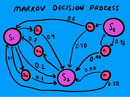
An MDP is a mathematical framework used for sequential decision-making problems, where an agent takes actions in an environment to maximize cumulative rewards.

🔹 Key Components of an MDP:

States (S) – A set of all possible situations in which the agent can be.
Actions (A) – A set of all actions available to the agent.
State Transition Probabilities (P) – Probability of moving from one state to another after taking an action.
Reward Function (R) – The numerical feedback the agent receives after taking an action.
Discount Factor (𝛾) – Determines the importance of future rewards.

🚀 Example: Self-Driving Car Navigation ✔ State: Car’s current location and surrounding traffic.
✔ Action: Accelerate, brake, turn left, turn right.
✔ Transition Probability: Probability of reaching a new location based on the action.
✔ Reward: Safe driving earns positive rewards; accidents yield negative rewards.

✅ MDPs help in modeling AI agents that must make sequential decisions in uncertain environments.

2. Agent-Environment Interaction in MDP

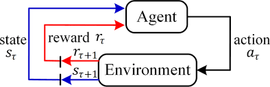
The Agent (decision-maker) interacts with the Environment by: 1️⃣ Observing the current state StS_tSt
2️⃣ Taking an action AtA_tAt
3️⃣ Receiving a reward RtR_tRt
4️⃣ Moving to the next state St+1S_{t+1}St+1

📌 Key Idea:
The goal of the agent is to learn an optimal policy π(a∣s)\pi(a|s)π(a∣s) that maximizes cumulative rewards over time.

3. Example: Grid World Problem

A Grid World is a simple MDP where:

The agent navigates a grid with walls and obstacles.
Actions include moving up, down, left, or right.
Some movements fail due to noise (e.g., intended “up” moves “left” instead).
Rewards:
- Small negative reward per step (battery consumption).
- Positive reward at the goal.
- Negative reward at failure states.

📌 Goal: The agent must learn an optimal policy to reach the goal while maximizing cumulative rewards.

✅ Grid World problems are widely used to illustrate MDP concepts and RL algorithms.

4. Policies in MDP: The Agent’s Decision-Making Rule

A policy π(a∣s)\pi(a|s)π(a∣s) defines the agent’s strategy at any given state.

🔹 Types of Policies:

Deterministic Policy – Always selects the same action for a given state. π(s)=a\pi(s) = aπ(s)=a
Stochastic Policy – Assigns probabilities to actions. π(a∣s)=P(At=a∣St=s)\pi(a|s) = P(A_t = a | S_t = s)π(a∣s)=P(At=a∣St=s)

🚀 Example: Traffic Light Control ✔ State: Number of waiting cars at an intersection.
✔ Actions: Change light timings dynamically.
✔ Policy: If congestion is high, extend the green signal.

✅ Learning an optimal policy is the core goal of reinforcement learning.

5. Value Functions: Measuring Future Rewards

MDPs use value functions to evaluate how good it is to be in a given state.

🔹 State-Value Function Vπ(s)V^\pi(s)Vπ(s)

Measures the expected return from state sss following policy π\piπ:Vπ(s)=Eπ[∑t=0∞γtRt∣S0=s]V^\pi(s) = E_\pi \left[ \sum_{t=0}^{\infty} \gamma^t R_t | S_0 = s \right]Vπ(s)=Eπ[t=0∑∞γtRt∣S0=s]

🔹 Action-Value Function Qπ(s,a)Q^\pi(s, a)Qπ(s,a)

Measures the expected return of taking action aaa in state sss:Qπ(s,a)=Eπ[∑t=0∞γtRt∣S0=s,A0=a]Q^\pi(s, a) = E_\pi \left[ \sum_{t=0}^{\infty} \gamma^t R_t | S_0 = s, A_0 = a \right]Qπ(s,a)=Eπ[t=0∑∞γtRt∣S0=s,A0=a]

📌 Key Insight:
The Bellman Equation expresses the recursive relationship between states and rewards.

✅ Value functions help agents evaluate the long-term benefits of actions.

6. Bellman Equations: The Heart of Dynamic Programming

The Bellman equation breaks down the value of a state into:

The immediate reward.
The discounted value of the next state.

Vπ(s)=∑aπ(a∣s)∑s′P(s′∣s,a)[R(s,a,s′)+γVπ(s′)]V^\pi(s) = \sum_a \pi(a|s) \sum_{s’} P(s’|s,a) [R(s,a,s’) + \gamma V^\pi(s’)]Vπ(s)=a∑π(a∣s)s′∑P(s′∣s,a)[R(s,a,s′)+γVπ(s′)]

🚀 Example: Chess AI Decision-Making ✔ State: Chessboard configuration.
✔ Action: Move a piece.
✔ Transition Probability: How likely the opponent responds in different ways.
✔ Reward: Winning the game vs. losing points.

✅ Bellman equations are fundamental to computing optimal policies.

7. Solving MDPs: Dynamic Programming (DP) Methods

To find the optimal policy, we use Dynamic Programming (DP) algorithms.

🔹 1. Value Iteration

1️⃣ Initialize V(s)=0V(s) = 0V(s)=0 for all states.
2️⃣ Iterate:V(s)=max⁡a∑s′P(s′∣s,a)[R(s,a,s′)+γV(s′)]V(s) = \max_a \sum_{s’} P(s’|s,a) [R(s,a,s’) + \gamma V(s’)]V(s)=amaxs′∑P(s′∣s,a)[R(s,a,s′)+γV(s′)]

3️⃣ Repeat until convergence.

✅ Value iteration computes the best value function and extracts an optimal policy.

🔹 2. Policy Iteration

1️⃣ Policy Evaluation: Compute Vπ(s)V^\pi(s)Vπ(s) for the current policy.
2️⃣ Policy Improvement: Update policy using:π(s)=arg⁡max⁡a∑s′P(s′∣s,a)[R(s,a,s′)+γVπ(s′)]\pi(s) = \arg\max_a \sum_{s’} P(s’|s,a) [R(s,a,s’) + \gamma V^\pi(s’)]π(s)=argamaxs′∑P(s′∣s,a)[R(s,a,s′)+γVπ(s′)]

3️⃣ Repeat until the policy converges.

✅ Policy iteration finds an optimal policy faster than value iteration.

8. Real-World Applications of MDPs

MDPs power AI-driven decision-making in various industries.

Industry	Application
Robotics	AI-powered robotic arms optimize motion planning.
Healthcare	AI selects optimal treatment plans for patients.
Finance	AI optimizes stock market investment strategies.
Self-Driving Cars	AI learns safe driving policies in dynamic environments.
Traffic Management	AI optimizes traffic light control to reduce congestion.

🚀 Example: AI in Healthcare ✔ AI decides when to administer medications based on patient history.
✔ MDPs model patient outcomes to optimize treatment plans.

✅ MDPs provide the foundation for real-world AI applications.

9. Conclusion: The Importance of MDPs in AI

MDPs formalize decision-making in uncertain environments, helping AI systems learn optimal policies.

🚀 Key Takeaways

✔ MDPs model sequential decision-making with uncertainty.
✔ Policies guide an agent’s actions to maximize cumulative rewards.
✔ Value functions measure the long-term benefits of states and actions.
✔ Bellman equations provide a recursive method to compute values.
✔ Dynamic Programming (Value Iteration & Policy Iteration) finds optimal policies.
✔ MDPs power AI applications in robotics, healthcare, and self-driving cars.

💡 What’s Next?
Future advancements will combine Deep Learning and MDPs to solve complex real-world AI challenges.

👉 How do you think MDPs will impact future AI developments? Let’s discuss in the comments! 🚀

This blog is structured, SEO-friendly, and optimized for AI and RL enthusiasts. Let me know if you need refinements! 🚀😊