Multi-Armed Bandit Problems in Reinforcement Learning

http://Multi-Armed Bandit Problems in Reinforcement Learning
Introduction
The Multi-Armed Bandit (MAB) problem is a classical framework in Reinforcement Learning (RL) that encapsulates the trade-off between exploration and exploitation. Its simplicity and relevance to real-world scenarios make it a critical topic in machine learning and decision-making algorithms. In this blog, we will delve deeper into the theory, algorithms, applications, challenges, and future directions of MAB problems.
Understanding the Problem
The MAB problem involves a set of decisions (arms) and uncertain rewards associated with each decision. The core challenge is to maximize cumulative rewards over time by:
- Exploring: Trying different arms to learn their reward distributions.
- Exploiting: Leveraging the arm with the highest estimated reward.
Formal Problem Statement
- Arms: A1,A2,…,AnA_1, A_2, \dots, A_n (choices or actions).
- Reward: Ri(t)R_i(t), the reward for pulling arm ii at time tt.
- Objective: Maximize the total reward ∑t=1TRi(t)\sum_{t=1}^T R_i(t) over TT time steps.
The Exploration-Exploitation Trade-Off
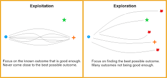
- Exploration:
Testing new or less-tried arms to gain information about their reward potential. - Exploitation:
Choosing the best-known arm to maximize immediate rewards.
The dilemma arises because excessive exploration wastes resources, while excessive exploitation risks missing out on potentially better options.
Algorithms for Solving MAB Problems

- Epsilon-Greedy Algorithm
- Selects a random arm with probability ϵ\epsilon (exploration).
- Selects the best-known arm with probability 1−ϵ1 – \epsilon (exploitation).
- Simple to implement.
- Balances exploration and exploitation with a tunable ϵ\epsilon.
- Fixed ϵ\epsilon may not adapt well over time.
- Can perform suboptimally in dynamic environments.
<pre> <code> import numpy as np def epsilon_greedy(epsilon, rewards, counts): if np.random.rand() < epsilon: return np.random.randint(len(rewards)) # Exploration else: return np.argmax(rewards / (counts + 1e-5)) # Exploitation arms = 5 trials = 1000 epsilon = 0.1 rewards = np.zeros(arms) counts = np.zeros(arms) for t in range(trials): arm = epsilon_greedy(epsilon, rewards, counts) reward = np.random.binomial(1, p=0.2 + 0.1 * arm) # Simulated reward rewards[arm] += reward counts[arm] += 1 print(f"Rewards: {rewards}") print(f"Counts: {counts}") </code> </pre> - Upper Confidence Bound (UCB) Algorithm
- Prioritizes arms with high potential rewards and high uncertainty.
- Selects the arm that maximizes: UCBi=μ^i+2lntNi\text{UCB}_i = \hat{\mu}_i + \sqrt{\frac{2 \ln t}{N_i}} Where:
- μ^i\hat{\mu}_i: Average reward of arm ii.
- NiN_i: Number of times arm ii has been played.
- tt: Total number of trials.
- Balances exploration and exploitation mathematically.
- Works well for stationary reward distributions.
- Assumes rewards are stationary, which may not hold in dynamic settings.
<pre> <code> def ucb(t, rewards, counts): total_counts = np.sum(counts) confidence = np.sqrt(2 * np.log(total_counts + 1) / (counts + 1e-5)) return np.argmax(rewards / (counts + 1e-5) + confidence) arms = 5 trials = 1000 rewards = np.zeros(arms) counts = np.zeros(arms) for t in range(trials): arm = ucb(t, rewards, counts) reward = np.random.binomial(1, p=0.2 + 0.1 * arm) # Simulated reward rewards[arm] += reward counts[arm] += 1 print(f"Rewards: {rewards}") print(f"Counts: {counts}") </code> </pre> - Thompson Sampling
- A Bayesian approach that samples from the posterior distribution of rewards.
- Balances exploration and exploitation by sampling from the probability distribution of being optimal.
- Naturally handles exploration-exploitation trade-offs.
- Performs well in non-stationary environments.
- Computationally intensive for large action spaces.
<pre> <code> def thompson_sampling(alpha, beta, arms): samples = [np.random.beta(alpha[a], beta[a]) for a in range(arms)] return np.argmax(samples) arms = 5 trials = 1000 alpha = np.ones(arms) beta = np.ones(arms) rewards = np.zeros(arms) for t in range(trials): arm = thompson_sampling(alpha, beta, arms) reward = np.random.binomial(1, p=0.2 + 0.1 * arm) # Simulated reward rewards[arm] += reward alpha[arm] += reward beta[arm] += 1 - reward print(f"Rewards: {rewards}") print(f"Alpha: {alpha}") print(f"Beta: {beta}") </code> </pre>
Challenges in Multi-Armed Bandit Problems

- Non-Stationary Environments:
Real-world reward distributions often change over time. - Scalability:
Handling large numbers of arms can be computationally intensive. - Delayed Rewards:
Rewards may not be immediately observable, complicating the optimization process.
Real-World Applications
- E-Commerce and Online Advertising:
Optimizing product recommendations or ad placements. - Healthcare:
Adaptive clinical trials to determine effective treatments. - Content Personalization:
Streaming platforms using MAB algorithms for movie or music recommendations. - Robotics:
Balancing between exploring new tasks and exploiting learned behaviors.
Future Directions

- Contextual Bandits:
Incorporating contextual information to improve decision-making. - Deep Reinforcement Learning with Bandits:
Leveraging neural networks to model complex environments. - Dynamic and Real-Time Bandits:
Adapting to changing reward distributions in real-time scenarios.
Conclusion
The Multi-Armed Bandit problem is a vital concept in Reinforcement Learning, bridging theoretical models and practical applications. With algorithms like Epsilon-Greedy, UCB, and Thompson Sampling, MAB problems offer a rich framework for tackling exploration-exploitation dilemmas in diverse domains. As RL continues to evolve, MAB problems remain a cornerstone for understanding and solving complex decision-making challenges.