A Comprehensive Overview of Parallelism in Machine Learning System Optimization 2024

A Comprehensive Overview of Parallelism in Machine Learning System Optimization 2024

Machine learning (ML) has entered an era where complex, data-intensive applications like deep learning, autonomous vehicles, and AI systems are at the forefront of technological development. These systems demand high processing power and low-latency computing, but the stagnation in single-threaded performance has made traditional methods of computation less effective. As a result, system designers are increasingly turning to parallel computing to address these challenges.

In this blog, we explore the fundamentals of parallelism in machine learning system optimization, the different types of parallel computing, and key concepts like concurrency, Amdahl’s Law, and Gustafson-Barsis’s Law, which help guide the optimization of ML applications for modern hardware architectures.

Understanding Parallelism and Concurrency

Before diving into parallel computing techniques, it is essential to differentiate between parallelism and concurrency:

• Concurrency refers to the composition of multiple computations into independent threads of execution. This concept is used when a system runs multiple tasks that are not necessarily executing simultaneously but may be running in overlapping periods. A typical example of concurrency is multiprogramming, where multiple tasks share a CPU to maximize resource utilization while one task waits for input/output (I/O).
• Parallelism, on the other hand, is the simultaneous execution of multiple computations. It aims to execute tasks in parallel to reduce latency and increase throughput by dividing a problem into smaller chunks that can be processed at the same time. In the context of ML, parallelism helps perform complex computations like gradient updates or matrix multiplications on multiple processors or GPUs simultaneously.

The Limits of Parallelism: Amdahl’s and Gustafson-Barsis’s Laws

While parallelism can significantly reduce latency, there are theoretical limits to how much performance improvement can be achieved, depending on the task’s characteristics:

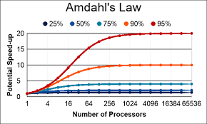
1. Amdahl’s Law: Amdahl’s Law highlights the theoretical speedup that can be achieved when parallelizing a program. The law emphasizes that even if a large portion of the program is parallelized, the remaining serial portion will act as a bottleneck and limit overall speedup. The formula for Amdahl’s Law is:Speedup=1(1−P)+PN\text{Speedup} = \frac{1}{(1 – P) + \frac{P}{N}}Speedup=(1−P)+NP​1​Where:
   • PPP is the parallelizable portion of the program,
   • NNN is the number of processors.
   This law suggests that even with high parallelism (e.g., 95% of a program is parallelizable), the speedup is constrained by the serial part. For instance, with a 95% parallelizable portion, the maximum theoretical speedup is 20x, which means the serial part still dictates performance limits.
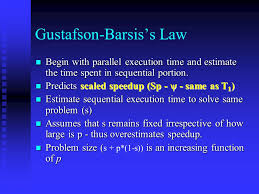
2. Gustafson-Barsis’s Law: For variable-sized problems, Gustafson-Barsis’s Law provides a more optimistic perspective on the limits of parallelism. This law suggests that when the problem size increases with the number of processors, the speedup can be linear, or even superlinear, due to the ability to scale the parallel workload. The formula for Gustafson-Barsis’s Law is:Speedup=N+(1−N)×s\text{Speedup} = N + (1 – N) \times sSpeedup=N+(1−N)×sWhere:
   • NNN is the number of processors,
   • sss is the serial portion of the program.
   This law shows that in real-world scenarios where the problem size increases with added computational resources, parallelism can offer near-linear speedup.

Sources of Parallelism

Parallelism can be extracted at various levels of computation, depending on the application and the hardware architecture. The following are the main sources of parallelism:

1. Bit-level Parallelism (BLP): This level of parallelism occurs within individual computations, such as when the CPU performs bitwise operations (e.g., addition, subtraction). BLP was more significant in earlier years but is now largely eclipsed by higher-level parallelism techniques.
2. Instruction-level Parallelism (ILP): ILP allows multiple independent instructions to execute in parallel. This is often achieved using out-of-order execution in modern processors. For example, superscalar CPUs can execute several instructions per cycle, improving performance by exploiting ILP.
3. Thread-level Parallelism (TLP): TLP enables multiple threads of execution to run concurrently. In systems with Simultaneous Multithreading (SMT) (e.g., Intel’s Hyper-Threading), the same physical core can execute multiple threads, increasing the CPU’s efficiency by filling idle times.
4. Accelerator-level Parallelism (ALP): In this case, specific tasks are offloaded to specialized hardware accelerators (e.g., GPUs, TPUs) designed to perform certain operations more efficiently than general-purpose CPUs.
5. Request-level Parallelism (RLP): RLP focuses on parallel processing of independent application requests. For example, in a distributed key-value store, multiple requests can be handled concurrently if they don’t depend on shared resources.

Parallel Computer Architectures

Parallel computing relies on different computer architectures that can be classified using Flynn’s Taxonomy:

1. SISD (Single Instruction, Single Data): The traditional serial architecture where a single instruction is executed on one data element at a time.
2. SIMD (Single Instruction, Multiple Data): Executes the same instruction on multiple data elements in parallel. Common in vector processors and GPUs.
3. MIMD (Multiple Instruction, Multiple Data): Involves multiple processors, each executing its own instruction stream on different data. This is typical in multicore processors.
4. MISD (Multiple Instruction, Single Data): Rare, but can be used for fault-tolerant systems where multiple instructions operate on the same data stream.
5. Systolic Architecture: A form of MIMD where data flows through a network of processors, with each processor performing simple tasks and passing intermediate results directly to the next processor.

Application and System Design: Shared Resources vs. Partitioned Resources

Parallel computing models can be further classified based on how resources are shared among processors:

1. Shared-Everything Approach: In this model, all processors have access to shared memory and resources, maximizing hardware utilization. However, it may face synchronization issues as multiple processors compete for resources.
2. Shared-Nothing Approach: Here, each processor has its own memory and resources. This eliminates synchronization overhead but may not fully utilize the system in cases where the workload is unevenly distributed.
3. Shared-Something Approach: This hybrid model uses shared resources within clusters of processors, combining the benefits of both shared-everything and shared-nothing approaches. It offers a balance between resource utilization and reduced synchronization overhead.

Task vs. Data Parallelism

When choosing how to parallelize an application, the decision between task parallelism and data parallelism is crucial. Task parallelism involves dividing the computation into independent tasks, while data parallelism divides the data and processes it in parallel. Understanding the task at hand and the program’s requirements will help developers select the optimal parallelism model for their workloads.

Conclusion: Maximizing Parallelism for High-Performance ML Systems

Parallel computing is an essential strategy for optimizing machine learning systems, especially as models and datasets continue to grow in size and complexity. By exploiting the various levels of parallelism, from instruction-level parallelism to thread-level parallelism and beyond, ML system designers can significantly improve performance, reduce latency, and maximize throughput.

The combination of understanding Amdahl’s Law and Gustafson-Barsis’s Law, along with efficient parallel programming models and system architectures, is key to achieving the best results in modern ML system optimization. As machine learning continues to push the boundaries of computational power, effective parallelism will remain a central focus for building scalable and efficient systems.