-Learning vs. Traditional Q-Learning: Key Differences and Advantages of Deep Neural Networks in RL
Introduction
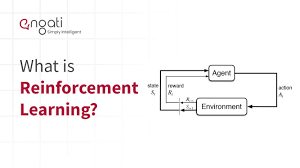
Reinforcement Learning (RL) is a rapidly evolving domain in Artificial Intelligence (AI) that enables agents to make sequential decisions in complex environments. Traditional algorithms like Q-Learning paved the way for RL but faced challenges in scalability and efficiency as environments grew in complexity. The advent of deep learning introduced a transformative approach—Deep Q-Learning (DQL)—that leverages deep neural networks to overcome these limitations.
In this blog, we will explore the fundamental differences between traditional Q-Learning and Deep Q-Learning, highlight the advantages of using deep neural networks in RL, and present code examples for better understanding.
What is Q-Learning?
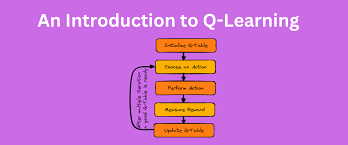
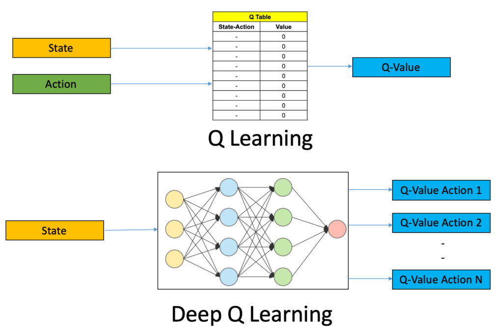
Q-Learning is one of the simplest and most foundational algorithms in reinforcement learning. It is a model-free, off-policy algorithm that aims to learn the optimal Q-Value function: Q(s,a)=Expected reward for taking action a in state s.Q(s, a) = \text{Expected reward for taking action } a \text{ in state } s.
Core Concepts in Q-Learning
- States (ss): Represent the environment’s conditions.
- Actions (aa): Choices the agent can make in a given state.
- Rewards (rr): Feedback received after taking an action.
- Q-Table: A lookup table storing Q-values for state-action pairs.
Q-Value Update Formula
The Q-value is updated iteratively using the Bellman Equation:
Q(s, a) = Q(s, a) + α [r + γ max Q(s', a') - Q(s, a)]
Where:
- αα = Learning rate
- γγ = Discount factor
- s′s’ = Next state
Limitations of Q-Learning
- State Explosion: The Q-Table grows exponentially with the state-action space.
- Lack of Generalization: Similar states are treated independently, leading to inefficiencies.
- Inability to Handle Continuous Spaces: Q-Learning struggles when states or actions are continuous, as tables cannot represent infinite possibilities.
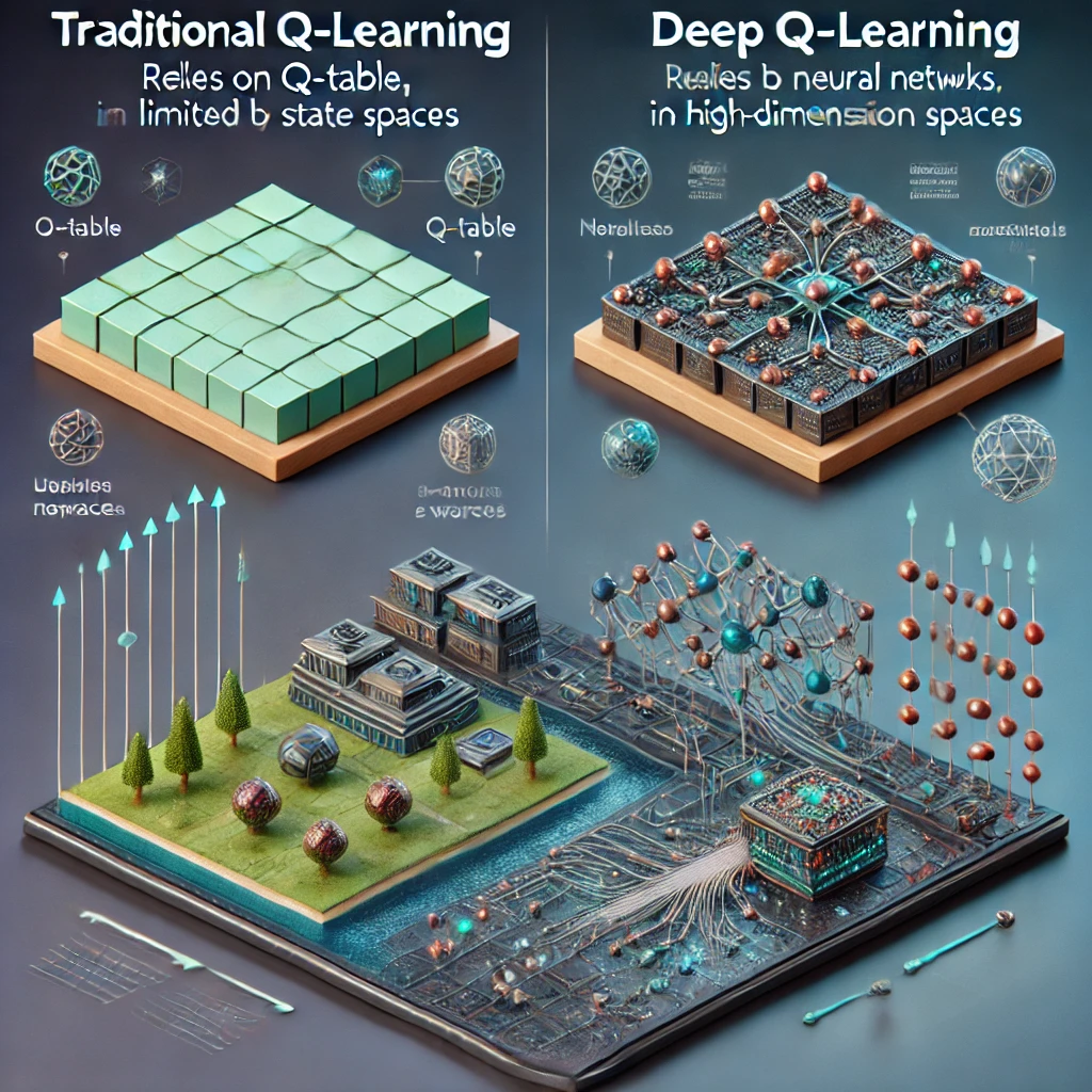
What is Deep Q-Learning (DQL)?
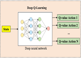
Deep Q-Learning addresses the limitations of Q-Learning by replacing the Q-Table with a Deep Neural Network (DNN). Instead of explicitly storing Q-values for all state-action pairs, the neural network approximates the Q-values using its weights and biases.
Architecture of Deep Q-Learning
- Input Layer: Represents the current state (ss).
- Hidden Layers: Extract features and learn patterns from input data.
- Output Layer: Outputs Q-values for all possible actions.
The DQL algorithm interacts with the environment to generate experience tuples: (s,a,r,s′)(s, a, r, s’)
These experiences are used to train the neural network, minimizing the loss function based on the Temporal Difference (TD) error.
Key Enhancements in Deep Q-Learning
- Experience Replay: Stores experiences in a replay buffer to break correlations between consecutive experiences, ensuring more stable learning.
- Target Network: Uses a separate target network to stabilize learning by providing fixed Q-value targets during updates.
- Batch Updates: Trains the neural network on mini-batches sampled from the replay buffer, improving sample efficiency.
The Loss Function in Deep Q-Learning
The loss function used to train the Q-Network is based on the Mean Squared Error (MSE) between the predicted Q-values and the target Q-values:
Loss = [r + γ max Q(s', a'; θ') - Q(s, a; θ)]²
Where:
- θθ = Parameters (weights) of the current Q-network.
- θ′θ’ = Parameters of the target Q-network.
Key Differences Between Q-Learning and Deep Q-Learning
| Aspect | Q-Learning | Deep Q-Learning |
|---|---|---|
| Q-Value Representation | Q-Table (explicit storage) | Neural Network (function approximation) |
| Scalability | Poor for large state spaces | Handles high-dimensional spaces effectively |
| Generalization | No generalization across states | Learns generalizable features |
| Handling Continuous Spaces | Not feasible | Easily adaptable |
| Computation | Computationally light but limited | Computationally intensive but powerful |
| Applications | Simple environments (e.g., gridworld) | Complex environments (e.g., video games) |
Advantages of Using Deep Neural Networks in RL
Deep neural networks offer several advantages that make them indispensable for modern reinforcement learning tasks:
1. Scalability
Deep Q-Learning can scale to environments with:
- Millions of states and actions.
- Continuous state or action spaces.
2. Generalization
Neural networks can generalize across similar states, enabling agents to learn efficiently even in sparse reward environments.
3. Automatic Feature Extraction
DNNs can automatically extract relevant features from raw data (e.g., images, sensor inputs), eliminating the need for manual feature engineering.
4. Handling Complex Problems
Deep Q-Learning has demonstrated success in solving problems that were previously considered infeasible, such as:
- Playing Atari games at a superhuman level.
- Controlling robotic arms in industrial settings.
- Navigating self-driving cars.
Advantages of Using Deep Neural Networks in RL
- Gaming
- DeepMind’s DQN achieved superhuman performance in Atari games.
- RL agents use pixel data as input and learn complex strategies.
- Robotics
- Teaching robots to perform tasks like picking and placing objects.
- Optimizing motion planning for efficient task execution.
- Autonomous Vehicles
- Real-time decision-making for navigation, obstacle avoidance, and control.
- Healthcare
- Optimizing treatment plans for personalized medicine.
- Designing adaptive prosthetics.
- Finance
- Portfolio optimization.
- Algorithmic trading.
Deep Q-Learning Example Code
Step 1: Building the Neural Network
<!DOCTYPE html>
<html>
<head>
    <title>Deep Q-Learning Example</title>
</head>
<body>
<pre>
# Import necessary libraries
import tensorflow as tf
from tensorflow.keras.models import Sequential
from tensorflow.keras.layers import Dense

# Build the Q-network
def build_q_network(state_size, action_size):
    model = Sequential([
        Dense(64, input_dim=state_size, activation='relu'),
        Dense(64, activation='relu'),
        Dense(action_size, activation='linear')
    ])
    model.compile(optimizer='adam', loss='mse')
    return model
</pre>
</body>
</html>
Step 2: Training the Agent
<!DOCTYPE html>
<html>
<head>
    <title>Training Loop Example</title>
</head>
<body>
<pre>
# Training loop
import numpy as np

# Parameters
gamma = 0.95  # Discount factor
epsilon = 1.0  # Exploration rate
epsilon_decay = 0.995
epsilon_min = 0.01

# Assume environment with state_size and action_size
state_size = 4  # Example state space
action_size = 2  # Example action space
q_network = build_q_network(state_size, action_size)

# Replay buffer
replay_buffer = []

# Add experience to replay buffer
def add_to_replay(state, action, reward, next_state, done):
    replay_buffer.append((state, action, reward, next_state, done))
    if len(replay_buffer) > 2000:  # Limit buffer size
        replay_buffer.pop(0)

# Sample batch and train
def train(batch_size):
    if len(replay_buffer) < batch_size:
        return
    mini_batch = np.random.choice(replay_buffer, batch_size, replace=False)
    for state, action, reward, next_state, done in mini_batch:
        target = reward
        if not done:
            target += gamma * np.max(q_network.predict(next_state))
        target_f = q_network.predict(state)
        target_f[0][action] = target
        q_network.fit(state, target_f, epochs=1, verbose=0)

# Example interaction with environment
state = np.random.rand(1, state_size)
for step in range(1000):  # Training steps
    if np.random.rand() <= epsilon:  # Exploration
        action = np.random.randint(action_size)
    else:  # Exploitation
        action = np.argmax(q_network.predict(state))

    # Take action in environment (example rewards)
    next_state = np.random.rand(1, state_size)
    reward = np.random.randint(1, 10)
    done = step == 999  # Episode ends at step 999

    # Add experience to replay buffer
    add_to_replay(state, action, reward, next_state, done)

    # Train on mini-batches
    train(batch_size=32)

    # Update state
    state = next_state

    # Decay exploration rate
    if epsilon > epsilon_min:
        epsilon *= epsilon_decay
</pre>
</body>
</html>
Challenges in Deep Q-Learning
- **Instability in Training
**: Overestimation of Q-values can lead to divergence. 2. High Resource Requirements: Training deep networks requires significant computational resources. 3. Hyperparameter Tuning: Requires careful tuning of learning rate, discount factor, and network architecture.
Conclusion
Deep Q-Learning revolutionizes traditional Q-Learning by leveraging the power of deep neural networks. This combination enables RL agents to scale to complex, high-dimensional environments, making them capable of solving real-world problems in gaming, robotics, and more. While challenges exist, advancements like experience replay and target networks ensure stable and efficient learning.
With Deep Q-Learning, the possibilities for AI agents in dynamic and complex environments are limitless!