comprehensive guide On-Policy Prediction with Function Approximation in Deep Reinforcement Learning 2024
Introduction
In Reinforcement Learning (RL), an agent interacts with an environment, learning to take actions that maximize rewards. However, traditional tabular learning methods struggle in complex environments where the state space is too large. Instead of storing values for each state, we use function approximation to generalize across similar states.
On-Policy Prediction with Approximation focuses on estimating value functions using function approximators like linear regression, deep neural networks, and gradient descent methods.
🚀 Why is Function Approximation Needed?
✔ Handles large state spaces efficiently
✔ Allows generalization to unseen states
✔ Speeds up learning by avoiding full state enumeration
✔ Works well with deep learning for complex tasks like robotics and gaming
✅ Instead of learning exact values for each state, RL models learn an approximation function that generalizes from experience.
1. Function Approximation in Reinforcement Learning
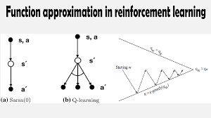
🔹 Traditional RL uses a value table to store state values, but in real-world problems, the number of states can be enormous or even infinite.
🔹 Instead, function approximation uses a mathematical function to estimate values for new, unseen states.
✅ Two Types of Function Approximation
| Type | Example | Use Case |
|---|---|---|
| Linear Approximation | Weighted sum of features | Simple, low-dimensional problems |
| Non-Linear Approximation | Deep Neural Networks (DNNs) | Complex tasks (robotics, image-based RL) |
🚀 Example: Self-Driving Cars
✔ A car learns how to navigate using features like speed, traffic, and road curves, rather than memorizing every road condition.
✅ Generalization allows RL agents to learn faster and adapt to new situations.
2. Stochastic Gradient Descent (SGD) in Function Approximation
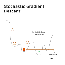
Gradient Descent is used to minimize the error in function approximation by adjusting the model’s parameters.
🔹 Steps in Gradient Descent for RL: 1️⃣ Compute the error between the predicted value and the actual return.
2️⃣ Update the weights using the gradient of the loss function.
3️⃣ Repeat until convergence.
🚀 Formula:wnew=wold−α⋅∇L(w)w_{new} = w_{old} – \alpha \cdot \nabla L(w) wnew=wold−α⋅∇L(w)
where:
✔ w = model weights
✔ α = learning rate
✔ ∇L(w) = gradient of the loss function
✅ SGD allows efficient updates, especially when handling large datasets in DRL.
3. Learning with Approximation: Q-Learning with Deep Networks
🔹 In Q-learning, the RL agent learns the value of state-action pairs to optimize decision-making.
🔹 Instead of storing all Q-values in a table, we use deep neural networks to approximate Q-values.
🚀 Example: Pac-Man AI ✔ A Q-learning agent in Pac-Man improves its strategy by approximating Q-values.
✔ Without approximation, it would take millions of episodes to memorize every possible game state.
✅ Deep Q-Networks (DQN) use neural networks to learn Q-values for large-scale RL problems.
4. On-Policy Learning with Function Approximation
On-Policy Learning means the agent improves the policy it is currently following.
🔹 Instead of using a separate exploratory policy, on-policy methods continuously refine the policy they are using.
✅ Two Main On-Policy Learning Methods
| Method | Description | Example |
|---|---|---|
| Monte Carlo (MC) Approximation | Learns from complete episodes | Episodic environments like games |
| Temporal Difference (TD) Learning | Updates values based on observed rewards and estimated future rewards | Real-time decision-making |
🚀 Example: Chess AI (On-Policy Learning) ✔ The AI continuously refines its game strategy as it plays, rather than training on a separate dataset.
✅ On-policy learning is useful for dynamic environments where strategies need real-time adaptation.
5. Semi-Gradient Methods in Deep Reinforcement Learning
🔹 Semi-gradient methods update the approximation function using both real and estimated rewards.
🚀 Why Use Semi-Gradient Methods? ✔ Faster convergence – Updates are made after each step, rather than waiting for an entire episode.
✔ More sample-efficient – Requires fewer interactions to learn optimal policies.
✅ Semi-gradient methods are widely used in Deep Q-Learning and Actor-Critic models.
6. Deep Q-Learning with Function Approximation
Deep Q-Learning extends traditional Q-learning by using a neural network to approximate Q-values.
🔹 Challenges in Deep Q-Learning: ✔ Overestimation Bias – The network might assign higher than expected Q-values.
✔ Non-Stationary Data – The training data distribution changes over time.
✔ Exploration-Exploitation Tradeoff – The agent must balance trying new actions vs. sticking to known good actions.
🚀 Solutions to Improve Deep Q-Learning
| Issue | Solution |
|---|---|
| Overestimation Bias | Use Double Deep Q-Networks (DDQN) |
| Non-Stationary Data | Use Experience Replay |
| Slow Convergence | Use Prioritized Experience Replay |
✅ Deep Q-Networks (DQN) improved state-of-the-art RL in video games like Atari and real-world applications.
7. Using Function Approximation in Monte Carlo Methods
Monte Carlo methods estimate the value function by averaging returns across episodes.
🔹 Why Use Monte Carlo with Function Approximation? ✔ Reduces variance in training.
✔ Works well in episodic environments (e.g., robotic grasping, games).
✔ More stable than pure temporal difference (TD) learning.
🚀 Example: AI in Board Games ✔ The AI samples thousands of possible game outcomes, refining its strategy over time.
✅ Monte Carlo methods combined with function approximation lead to robust decision-making in long-term planning problems.
8. Feature Engineering for Function Approximation
🔹 In RL, instead of using raw states, we extract meaningful features to improve learning efficiency.
✅ Feature Engineering Methods in RL
| Method | Use Case |
|---|---|
| Coarse Coding | Groups similar states together for efficient learning |
| Tile Coding | Divides the state space into overlapping regions |
| Radial Basis Functions (RBFs) | Useful for continuous state spaces |
🚀 Example: Autonomous Drone Navigation ✔ Instead of learning exact coordinates, the drone learns abstract flight patterns, reducing complexity.
✅ Feature engineering accelerates learning in complex RL environments.
9. Summary and Key Takeaways
On-policy function approximation helps RL agents generalize across large state spaces, improving efficiency and learning speed.
✅ Key Takeaways
✔ Function approximation generalizes RL models to unseen states.
✔ Deep networks enable scalable Q-learning in large environments.
✔ Gradient descent is essential for tuning approximation functions.
✔ On-policy learning refines strategies in real-time environments.
✔ Feature engineering improves efficiency in complex RL tasks.
💡 Which function approximation method have you used in reinforcement learning? Let’s discuss in the comments! 🚀
Would you like a step-by-step tutorial on implementing function approximation in RL using TensorFlow? 😊