The Curse of Dimensionality in Dynamic Programming and the Role of Function Approximation Techniques 2024
In the world of machine learning and reinforcement learning, dynamic programming (DP) has become a key technique for solving decision-making problems. However, one significant challenge that arises when applying DP to complex environments is the curse of dimensionality. This phenomenon makes traditional methods of dynamic programming intractable for many real-world problems. Fortunately, function approximation techniques provide a way to mitigate this issue, allowing us to tackle problems with high-dimensional state or action spaces more efficiently. In this blog, we will explore the curse of dimensionality in dynamic programming, how it affects decision-making problems, and how function approximation techniques can help overcome these challenges.
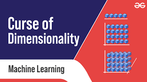
What is the Curse of Dimensionality?
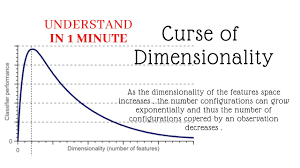
The curse of dimensionality refers to the exponential increase in computational resources required as the number of dimensions (or features) in a problem increases. In the context of dynamic programming, this term describes the rapid growth of the state and action space as the problem size increases, making it computationally expensive to store and process the required information.
In Dynamic Programming
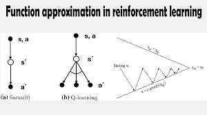
Dynamic programming is a method used to solve problems by breaking them down into smaller subproblems and solving them recursively. In reinforcement learning and optimal control problems, DP is used to find the optimal policy, which maps each state to the best action to take in order to maximize cumulative rewards.
When applying DP to problems with Markov Decision Processes (MDPs), the state and action spaces can grow rapidly as the number of state variables and actions increases. For example, consider a grid-world environment where each state corresponds to a specific position on the grid. As the grid size increases, the number of possible states increases exponentially. This leads to an explosion in the number of state-action pairs the agent must evaluate in order to find the optimal policy.
For a problem with NN state variables, if each state variable has SS possible values, the total number of states is SNS^N. The curse of dimensionality emerges as this number increases significantly with the growth of NN, making it infeasible to apply traditional dynamic programming algorithms (such as value iteration or policy iteration) that require evaluating every state-action pair.
Key Challenges of the Curse of Dimensionality in DP

- State Explosion: As the dimensionality of the state space increases, the number of states increases exponentially, making it impractical to store and compute values for each state.
- Action Explosion: In many problems, there is not only a large number of states but also a large number of actions to choose from. This leads to an even greater explosion in the number of state-action pairs that must be evaluated.
- Computational Intractability: As the number of states and actions grows, the time and memory required to store and compute values for all states becomes computationally intractable, even with the most efficient algorithms.
- Memory Limitations: Storing large value tables (like state-value or action-value tables) requires large amounts of memory. This is especially problematic in high-dimensional state or action spaces.
Function Approximation Techniques: A Solution to the Curse of Dimensionality
Function approximation techniques provide a way to address the curse of dimensionality by approximating the value functions (state-value or action-value functions) instead of storing them explicitly for every possible state or state-action pair. These techniques allow the agent to generalize from a smaller number of examples, thereby reducing the complexity and memory requirements of the problem.
What is Function Approximation?
Function approximation involves approximating the value function using a parametric model, such as a neural network, linear function, or decision tree. Instead of storing the value for every state or state-action pair, the agent uses a function to predict values for unseen states or actions. The function is learned through training, where the goal is to minimize the error between the predicted values and the true values (or estimated values based on experience).
Types of Function Approximation
- Linear Function Approximation:
- A simple form of function approximation involves using a linear combination of features of the state or state-action pair. For instance, if a state is represented by a vector of features ϕ(s)\phi(s), the value function can be approximated as:
- Polynomial and Non-linear Function Approximation:
- For more complex problems, linear functions may not be sufficient. Non-linear function approximation (e.g., neural networks, decision trees) allows for more flexible models that can capture intricate patterns in the data.
- In reinforcement learning, deep Q-networks (DQN) use neural networks to approximate the Q-value function, enabling the agent to handle high-dimensional state spaces like those encountered in video games and robotics.
- K-Nearest Neighbors (KNN) and Similar Techniques:
- Other function approximation techniques, such as KNN or kernel methods, can also be used to approximate value functions. These techniques work by identifying similar states or actions and using their values to estimate the value of the current state.
How Function Approximation Helps Mitigate the Curse of Dimensionality
1. Reduced Memory Requirements
Function approximation reduces the need to store a large table of values for every state or state-action pair. Instead of explicitly storing values for each combination, we store the parameters of the approximation function, which significantly reduces memory requirements. In high-dimensional environments, such as video games or robotic control, this is crucial for making problems tractable.
For instance, a neural network can learn to generalize across many states, enabling the agent to predict the value of unseen states based on learned patterns.
2. Generalization Across States
Function approximation allows an agent to generalize the value of one state to similar states. For example, in a grid-world problem, if the agent learns the value of a specific state, it may be able to approximate the values of nearby states with similar characteristics, without having to compute each one individually. This drastically reduces the number of calculations needed and improves the efficiency of the learning process.
3. Scalability to High-Dimensional Spaces
As the number of states and actions increases, the complexity of the problem grows exponentially. With function approximation, the agent can handle much higher-dimensional spaces by learning a mapping from states to values using a smaller set of features. This is especially useful when dealing with environments that have continuous or very large state spaces, such as robot navigation, video game environments, or financial modeling.
For example, in Deep Reinforcement Learning (DRL), function approximation using neural networks allows the agent to handle high-dimensional input spaces, like raw pixels in a video game, where traditional methods would fail due to the curse of dimensionality.
4. Improved Convergence Rates
By approximating value functions, function approximation techniques can improve the convergence rates of dynamic programming algorithms. This is because they help the agent learn from broader patterns in the state space, allowing it to converge more quickly to an optimal policy without having to evaluate every state or state-action pair individually.
Practical Example: Deep Q-Learning
Deep Q-Learning is a reinforcement learning algorithm that uses a neural network to approximate the action-value function Q(s,a)Q(s, a). Instead of maintaining a table of Q-values for every state-action pair, DQN uses a neural network to approximate the Q-function based on the current state and action.
Code Example: Deep Q-Learning with Function Approximation
Here is a simple implementation of Deep Q-Learning using function approximation:
import numpy as np
import tensorflow as tf
from tensorflow.keras import layers
import random

# Define the environment
class SimpleEnv:
    def __init__(self):
        self.state_space = 4
        self.action_space = 2
        self.state = np.zeros(self.state_space)

    def reset(self):
        self.state = np.random.rand(self.state_space)
        return self.state

    def step(self, action):
        next_state = self.state + np.random.rand(self.state_space) * action  # simple environment dynamics
        reward = -np.linalg.norm(next_state)  # reward is negative of distance from origin
        done = np.linalg.norm(next_state) < 0.1
        return next_state, reward, done

# Define the neural network model for function approximation
def build_model(state_space, action_space):
    model = tf.keras.Sequential([
        layers.Dense(64, input_dim=state_space, activation='relu'),
        layers.Dense(64, activation='relu'),
        layers.Dense(action_space, activation='linear')  # Q-values for each action
    ])
    model.compile(optimizer='adam', loss='mse')
    return model

# Q-learning with function approximation (DQN)
class DQNAgent:
    def __init__(self, state_space, action_space, gamma=0.95, epsilon=0.1, alpha=0.01):
        self.state_space = state_space
        self.action_space = action_space
        self.gamma = gamma
        self.epsilon = epsilon
        self.alpha = alpha
        self.model = build_model(state_space, action_space)
        self.memory = []

    def act(self, state):
        if np.random.rand() < self.epsilon:
            return np.random.randint(self.action_space)  # explore
        else:
            q_values = self.model.predict(state.reshape(1, -1))  # predict Q-values for all actions
            return np.argmax(q_values)  # exploit

    def remember(self, state, action, reward, next_state, done):
        self.memory.append((state, action, reward
, next_state, done))
def replay(self, batch_size=32):
    if len(self.memory) < batch_size:
        return

    batch = random.sample(self.memory, batch_size)

    for state, action, reward, next_state, done in batch:
        target = reward
        if not done:
            target += self.gamma * np.max(self.model.predict(next_state.reshape(1, -1)))
        q_values = self.model.predict(state.reshape(1, -1))
        q_values[0][action] = target
        self.model.fit(state.reshape(1, -1), q_values, epochs=1, verbose=0)
Training the DQN agent
env = SimpleEnv() agent = DQNAgent(state_space=4, action_space=2)
for episode in range(1000): state = env.reset() done = False while not done: action = agent.act(state) next_state, reward, done = env.step(action) agent.remember(state, action, reward, next_state, done) state = next_state agent.replay(batch_size=32)
if episode % 100 == 0:
    print(f"Episode {episode} complete.")
In this code:
- The agent interacts with a simple environment where it takes actions and receives rewards.
- The agent uses a neural network (function approximation) to approximate the Q-values for state-action pairs, rather than storing a table of Q-values for all state-action pairs.
- The model learns to approximate the optimal policy through experience replay, updating the Q-values based on the agent's actions and rewards.

---

## Conclusion

The curse of dimensionality is one of the major challenges faced when applying dynamic programming to real-world problems. As the dimensionality of the state and action spaces increases, traditional DP methods become computationally intractable. However, function approximation techniques, particularly through methods like neural networks, offer a powerful solution. By approximating value functions, agents can generalize across states and actions, drastically reducing memory requirements and making it feasible to handle high-dimensional problems efficiently.

As reinforcement learning continues to advance, the use of function approximation will remain critical for solving increasingly complex decision-making tasks. From robotic control to game playing and autonomous systems, function approximation techniques provide the flexibility and scalability needed to tackle some of the most exciting challenges in artificial intelligence today.
Conclusion
The curse of dimensionality is one of the major challenges faced when applying dynamic programming to real-world problems. As the dimensionality of the state and action spaces increases, traditional DP methods become computationally intractable. However, function approximation techniques, particularly through methods like neural networks, offer a powerful solution. By approximating value functions, agents can generalize across states and actions, drastically reducing memory requirements and making it feasible to handle high-dimensional problems efficiently.
As reinforcement learning continues to advance, the use of function approximation will remain critical for solving increasingly complex decision-making tasks. From robotic control to game playing and autonomous systems, function approximation techniques provide the flexibility and scalability needed to tackle some of the most exciting challenges in artificial intelligence today.