The Exploration-Exploitation Trade-off in Reinforcement Learning

http://The Exploration-Exploitation Trade-off in Reinforcement Learning
Reinforcement Learning (RL) is a subset of machine learning where an agent interacts with an environment to learn optimal actions. A key challenge in RL is managing the exploration-exploitation trade-off. This concept is at the heart of many RL algorithms and plays a vital role in achieving long-term success in dynamic, uncertain environments.
In this comprehensive blog, we will delve deeper into the theory, strategies, applications, and real-world examples of the exploration-exploitation trade-off, along with code samples to solidify your understanding.
What is the Exploration-Exploitation Trade-off?
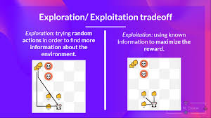
At its core, this trade-off involves balancing:
- Exploration: Trying out new or less-frequently used actions to gather more information about their outcomes. This step helps the agent discover potentially better strategies.
- Exploitation: Leveraging the known information to maximize immediate rewards by selecting the best-known actions.
This trade-off is not just theoretical; it reflects real-life decision-making challenges. For instance:
- In marketing: Should a company continue spending on existing, proven strategies or try new advertising channels?
- In career planning: Should an individual stay in a stable job or explore new, potentially riskier opportunities?
Reinforcement Learning algorithms aim to formalize and solve this dilemma in a computational framework.
Why Does This Trade-off Matter?
The trade-off is critical because:
- Optimal Learning: Pure exploitation leads to suboptimal learning. Without exploration, the agent might miss discovering better strategies. For instance, in a multi-armed bandit problem, the agent might settle for a seemingly high-reward arm while neglecting a better arm that requires exploration.
- Efficiency: Uncontrolled exploration can waste resources. If the agent spends excessive time exploring, it delays achieving optimal rewards.
- Dynamic Environments: In real-world scenarios where environments change (e.g., stock markets), continuous exploration ensures the agent adapts and stays relevant.
Theoretical Insights
In mathematical terms, the exploration-exploitation trade-off is often expressed as balancing expected reward (exploitation) with uncertainty reduction (exploration). Consider a Markov Decision Process (MDP), where:
- SS: Set of states
- AA: Set of actions
- P(s′∣s,a)P(s’|s, a): Probability of transitioning to state s′s’ after taking action aa in state ss
- R(s,a)R(s, a): Reward for taking action aa in state ss
The agent’s goal is to maximize the cumulative discounted reward: Gt=Rt+γRt+1+γ2Rt+2+…G_t = R_t + \gamma R_{t+1} + \gamma^2 R_{t+2} + \dots
where γ\gamma is the discount factor. Balancing exploration and exploitation is critical for identifying the optimal policy π(s)\pi(s) that determines the best action in each state.
Real-World Examples of Exploration-Exploitation
- Web Personalization:
- Exploration: Testing new layouts or recommendation algorithms for users.
- Exploitation: Showing content that has consistently performed well.
- Drug Discovery:
- Exploration: Trying new combinations of molecules to find effective drugs.
- Exploitation: Using known combinations that have shown good results.
- Autonomous Vehicles:
- Exploration: Testing alternative routes to learn traffic patterns.
- Exploitation: Taking the fastest known route.
- Online Advertising:
- Exploration: Displaying new ads to assess user engagement.
- Exploitation: Using ads with proven click-through rates.
Strategies for Managing the Trade-off
1. ε-Greedy Strategy
This is one of the simplest and most commonly used strategies. The agent chooses a random action (exploration) with probability ϵ\epsilon and the best-known action (exploitation) with probability 1−ϵ1-\epsilon.
Advantages:
- Easy to implement.
- Works well in many practical scenarios.
Disadvantages:
- Exploration is uniform; it doesn’t consider the uncertainty of actions.
Code Implementation:
import random

def epsilon_greedy(Q, state, epsilon):
    if random.uniform(0, 1) < epsilon:
        # Explore
        return random.choice(list(Q[state].keys()))
    else:
        # Exploit
        return max(Q[state], key=Q[state].get)
2. Decaying ε-Greedy
To improve ε-Greedy, we can reduce ϵ\epsilon over time. Initially, the agent explores extensively, but as it learns more, it shifts focus to exploitation.
Advantages:
- Balances exploration and exploitation over time.
- Suitable for environments that don’t change significantly.
Code Example:
epsilon = 1.0  # Start with high exploration
decay_rate = 0.995
min_epsilon = 0.01

for episode in range(1000):
    epsilon = max(min_epsilon, epsilon * decay_rate)
    action = epsilon_greedy(Q, state, epsilon)
3. Upper Confidence Bound (UCB)
UCB selects actions based on both their estimated value and the uncertainty associated with them. Actions with higher uncertainty are explored more.
Formula: UCB(a)=Q(a)+c⋅lnNNaUCB(a) = Q(a) + c \cdot \sqrt{\frac{\ln N}{N_a}}
Where:
- Q(a)Q(a): Estimated value of action aa
- NN: Total number of trials
- NaN_a: Number of times action aa has been selected
- cc: Exploration parameter
Code Implementation:
import math

def ucb(Q, N, total_steps, state):
    values = []
    for a in range(len(Q[state])):
        if N[state][a] > 0:
            ucb_value = Q[state][a] + math.sqrt(2 * math.log(total_steps) / N[state][a])
        else:
            ucb_value = float('inf')  # Ensure unexplored actions are prioritized
        values.append(ucb_value)
    return values.index(max(values))
4. Thompson Sampling
Thompson Sampling models the uncertainty of action rewards using probability distributions. It selects actions by sampling from these distributions.
Advantages:
- Provides a principled way to balance exploration and exploitation.
- Works well in environments with stochastic rewards.
Challenges and Limitations
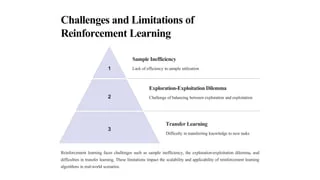
- Dynamic Environments: When environments change rapidly, static strategies like ε-Greedy may fail.
- Computational Complexity: Advanced strategies like UCB and Thompson Sampling can be computationally expensive.
- Delayed Rewards: In some scenarios, actions may yield rewards only after significant delays, complicating exploration.
Advanced Topics
Bayesian Reinforcement Learning
Bayesian RL explicitly incorporates uncertainty into the model by maintaining a posterior distribution over the reward function or transition probabilities. It optimizes the exploration-exploitation trade-off more effectively but at a higher computational cost.
Contextual Bandits
A contextual bandit is an extension of the multi-armed bandit problem where additional context (features) is available for decision-making. This is widely used in recommendation systems and ad placement.
Practical Example: Balancing Exploration and Exploitation
Here’s an example of the Multi-Armed Bandit problem implemented using the ε-Greedy strategy:
import numpy as np

# Simulated rewards for 3 arms
true_rewards = [0.2, 0.5, 0.7]  # True probabilities of success
arms = len(true_rewards)
Q = np.zeros(arms)  # Estimated rewards
N = np.zeros(arms)  # Number of pulls for each arm
epsilon = 0.1  # Exploration probability
total_steps = 1000

for step in range(total_steps):
    if np.random.rand() < epsilon:
        # Exploration
        action = np.random.choice(arms)
    else:
        # Exploitation
        action = np.argmax(Q)

    # Simulate reward
    reward = 1 if np.random.rand() < true_rewards[action] else 0
    N[action] += 1
    Q[action] += (reward - Q[action]) / N[action]  # Update Q value

print("Estimated rewards:", Q)
Visualizing the Trade-off
A simple plot can help illustrate how ε decays over time:
import matplotlib.pyplot as plt

epsilon = 1.0
decay_rate = 0.995
min_epsilon = 0.01
epsilons = []

for episode in range(1000):
    epsilon = max(min_epsilon, epsilon * decay_rate)
    epsilons.append(epsilon)

plt.plot(epsilons)
plt.title("Epsilon Decay Over Episodes")
plt.xlabel("Episodes")
plt.ylabel("Epsilon (Exploration Probability)")
plt.show()
Applications Across Industries
- Finance: Portfolio optimization using exploration to identify emerging markets.
- Healthcare: Personalized treatments by exploring less-tested therapies.
- E-commerce: Recommender systems that explore new products and exploit user preferences.
Conclusion
The exploration-exploitation trade-off is fundamental in Reinforcement Learning and real-world decision-making. Understanding its principles and applying strategies like ε-Greedy, UCB, and Thompson Sampling can lead to efficient learning and better performance. While it poses challenges in dynamic environments, advanced techniques such as Bayesian RL and