Dynamic Programming and Its Role in Solving Markov Decision Processes (MDPs) 2024

Dynamic Programming and Its Role in Solving Markov Decision Processes (MDPs)

http://Dynamic Programming and Its Role in Solving Markov Decision Processes (MDPs) 2024

Dynamic programming (DP) is a mathematical optimization and algorithmic technique used to solve problems by breaking them down into simpler subproblems and solving each subproblem just once, storing its solution for future reference. This technique is especially powerful for solving sequential decision-making problems, such as Markov Decision Processes (MDPs).

This blog will cover dynamic programming, its principles, and its critical relationship with solving MDPs. We’ll include theoretical explanations, examples, and code in an HTML editor format for easy use.

Introduction to Dynamic Programming
Key Concepts of Dynamic Programming
Introduction to Markov Decision Processes
Dynamic Programming and MDPs
- Policy Evaluation
- Policy Improvement
- Policy Iteration
- Value Iteration
Applications of DP in MDPs
Advantages and Limitations
Conclusion

1. Introduction to Dynamic Programming

Dynamic programming is based on two key principles:

Optimal Substructure: The problem can be divided into smaller, overlapping subproblems.
Memoization or Tabulation: The solutions to these subproblems are stored to avoid redundant computations.

Dynamic programming can be applied to problems with deterministic or stochastic transitions, making it a natural fit for solving MDPs.

2. Key Concepts of Dynamic Programming

2.1 Bellman Equation

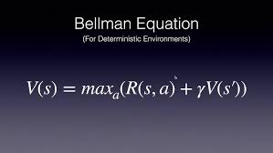
At the heart of DP is the Bellman Equation, which provides a recursive formulation to compute the optimal value function for decision-making.

For a state ss in an MDP: V(s)=max⁡a[R(s,a)+γ∑s′P(s′∣s,a)V(s′)]V(s) = \max_a \left[ R(s, a) + \gamma \sum_{s’} P(s’|s, a) V(s’) \right]

Where:

V(s)V(s) is the value of state ss.
R(s,a)R(s, a) is the immediate reward for taking action aa in state ss.
γ\gamma is the discount factor (0≤γ≤10 \leq \gamma \leq 1).
P(s′∣s,a)P(s’|s, a) is the transition probability to state s′s’ from state ss given action aa.

2.2 Dynamic Programming Algorithms

The two main DP algorithms for solving MDPs are:

Policy Iteration
Value Iteration

3. Introduction to Markov Decision Processes (MDPs)

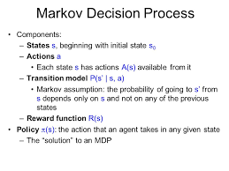
An MDP is a mathematical framework for modeling decision-making where outcomes are partly random and partly under the control of a decision-maker. It is defined by:

States (SS): A finite set of states.
Actions (AA): A finite set of actions available to the agent.
Transition Probabilities (P(s′∣s,a)P(s’|s, a)): Probability of moving to state s′s’ from ss after action aa.
Rewards (R(s,a)R(s, a)): The immediate reward received after taking action aa in state ss.
Discount Factor (γ\gamma): Determines the importance of future rewards.

The goal of solving an MDP is to find a policy π\pi that maximizes the expected cumulative reward.

4. Dynamic Programming and MDPs

4.1 Policy Evaluation

Policy evaluation computes the value of each state under a specific policy π\pi: Vπ(s)=∑aπ(a∣s)[R(s,a)+γ∑s′P(s′∣s,a)Vπ(s′)]V^\pi(s) = \sum_a \pi(a|s) \left[ R(s, a) + \gamma \sum_{s’} P(s’|s, a) V^\pi(s’) \right]

Code:

<!DOCTYPE html>
<html>
<head>
    <title>Policy Evaluation</title>
</head>
<body>
<pre>
# Python Implementation of Policy Evaluation
import numpy as np

def policy_evaluation(policy, P, R, gamma, theta=1e-6):
    """
    Evaluate a given policy.
    Args:
        policy: A matrix of size SxA, where each entry policy[s][a] is the probability of taking action a in state s.
        P: Transition probabilities, a 3D array P[s][a][s'].
        R: Rewards, a 2D array R[s][a].
        gamma: Discount factor.
        theta: Convergence threshold.
    Returns:
        V: Value function for the given policy.
    """
    num_states = len(P)
    V = np.zeros(num_states)
    while True:
        delta = 0
        for s in range(num_states):
            v = V[s]
            V[s] = sum(policy[s][a] * (R[s][a] + gamma * sum(P[s][a][s_] * V[s_] for s_ in range(num_states)))
                       for a in range(len(policy[s])))
            delta = max(delta, abs(v - V[s]))
        if delta < theta:
            break
    return V
</pre>
</body>
</html>

4.2 Policy Improvement

Policy improvement updates the policy based on the value function to ensure better rewards: π′(s)=arg⁡max⁡a[R(s,a)+γ∑s′P(s′∣s,a)Vπ(s′)]\pi'(s) = \arg\max_a \left[ R(s, a) + \gamma \sum_{s’} P(s’|s, a) V^\pi(s’) \right]

4.3 Policy Iteration

Policy iteration alternates between policy evaluation and improvement until convergence. It guarantees finding the optimal policy in finite steps.

4.4 Value Iteration

Value iteration simplifies the process by directly updating the value function: V(s)=max⁡a[R(s,a)+γ∑s′P(s′∣s,a)V(s′)]V(s) = \max_a \left[ R(s, a) + \gamma \sum_{s’} P(s’|s, a) V(s’) \right]

Code:

<!DOCTYPE html>
<html>
<head>
    <title>Value Iteration</title>
</head>
<body>
<pre>
# Python Implementation of Value Iteration
def value_iteration(P, R, gamma, theta=1e-6):
    """
    Solve MDP using Value Iteration.
    Args:
        P: Transition probabilities, a 3D array P[s][a][s'].
        R: Rewards, a 2D array R[s][a].
        gamma: Discount factor.
        theta: Convergence threshold.
    Returns:
        V: Optimal value function.
        policy: Optimal policy.
    """
    num_states, num_actions = len(P), len(P[0])
    V = np.zeros(num_states)
    while True:
        delta = 0
        for s in range(num_states):
            v = V[s]
            V[s] = max(R[s][a] + gamma * sum(P[s][a][s_] * V[s_] for s_ in range(num_states))
                      for a in range(num_actions))
            delta = max(delta, abs(v - V[s]))
        if delta < theta:
            break

primary algorithms in dynamic programming are:

Policy Iteration

Involves two main steps:
1. Policy Evaluation: Calculate the value function for a given policy.
2. Policy Improvement: Update the policy to maximize rewards based on the evaluated value function.

Value Iteration

Directly computes the optimal value function by iteratively updating the value estimates based on the Bellman equation, without explicitly evaluating a policy at every step.

5. Applications of DP in MDPs

Dynamic programming techniques are widely used in:

Robotics: Navigation and path planning.
Finance: Portfolio optimization.
Healthcare: Treatment planning.
Games: AI decision-making (e.g., chess, Go).

6. Advantages and Limitations

Advantages

Guarantees an optimal solution for MDPs.
Systematic approach to solving complex sequential problems.

Limitations

Computationally expensive for large state spaces.
Memory-intensive due to the need to store value functions and policies.

7. Conclusion

Dynamic programming is a powerful technique for solving Markov Decision Processes. By leveraging principles like the Bellman equation, it allows systematic optimization of policies and value functions. While computationally intensive, its structured approach guarantees optimal solutions in a variety of domains.

This blog provides a solid foundation to understand the synergy between DP and MDPs, with practical examples and code to help you dive deeper into real-world applications.