Optimization in Deep Neural Networks: Techniques and Best Practices 2024

Optimization in Deep Neural Networks: Techniques and Best Practices 2024

Introduction

Optimization is a critical step in training Deep Neural Networks (DNNs). The choice of optimization algorithm impacts convergence speed, accuracy, and generalization.

🚀 Why is Optimization Important in Deep Learning?

✔ Ensures efficient training and convergence
✔ Helps escape local minima and saddle points
✔ Prevents vanishing and exploding gradients
✔ Optimizes learning rate for faster convergence

In this guide, we’ll cover:
✅ Challenges in neural network optimization
✅ Gradient-based optimization techniques
✅ Adaptive learning rate algorithms
✅ Momentum-based optimization methods

---

1. Challenges in Deep Learning Optimization

Optimizing deep networks is challenging due to non-convex loss surfaces. Major challenges include:

🔹 Local Minima – The model gets stuck in a suboptimal point.
🔹 Saddle Points – Points where gradients vanish, slowing training.
🔹 Vanishing & Exploding Gradients – Early layers fail to learn due to extreme weight updates.

🚀 Example:
A DNN trained for image classification may struggle to find the global minimum due to the complexity of the loss function landscape.

✅ Solution:
Advanced optimizers like Momentum, Adam, and RMSProp help escape saddle points and speed up training.

---

2. Gradient-Based Optimization: Gradient Descent

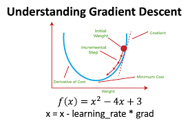
Gradient Descent (GD) is the foundation of deep learning optimizers. It updates weights iteratively to minimize the loss function.

🔹 Gradient Descent Update Rule:wnew=wold−η∗∇L(w)w_{new} = w_{old} – \eta * \nabla L(w) wnew​=wold​−η∗∇L(w)

where:

• w = model weights
• η (eta) = learning rate
• ∇L(w) = gradient of the loss function

✅ Types of Gradient Descent

Type	Description	Use Case
Batch GD	Uses the full dataset for each update	Slow, but precise
Stochastic GD (SGD)	Updates weights after each training sample	Noisy but faster
Mini-Batch GD	Updates weights in small batches	Best trade-off

🚀 Example:
SGD is widely used for large-scale image recognition as it improves speed and efficiency.

✅ Best Practice: Use Mini-Batch GD for a balance of speed and stability.

---

3. Learning Rate: The Key Hyperparameter

The learning rate (η) controls how much weights change per update.

🔹 Effects of Learning Rate: ✔ Too Small → Training is slow, stuck in local minima.
✔ Too Large → Training oscillates, may never converge.

🚀 Example:
For an NLP model, setting η = 0.0001 might be too slow, while η = 1.0 can cause divergence.

✅ Solution: Use adaptive learning rate optimizers like Adam or RMSProp.

---

4. Momentum-Based Optimization

Momentum helps models accelerate in the right direction and dampens oscillations.

🔹 Momentum Update Rule:vt=β∗vt−1+η∗∇L(w)wnew=wold−vtv_{t} = β * v_{t-1} + η * ∇L(w) w_{new} = w_{old} – v_{t} vt​=β∗vt−1​+η∗∇L(w)wnew​=wold​−vt​

where:

• β (beta) = momentum coefficient (typically 0.9).

🚀 Example: Image Recognition ✔ Without momentum: Training gets stuck at saddle points.
✔ With momentum: The optimizer pushes through plateaus for faster convergence.

✅ Momentum accelerates training and prevents getting stuck in local minima.

---

5. Adaptive Learning Rate Algorithms

Unlike SGD, which uses a fixed learning rate, adaptive optimizers adjust learning rates dynamically.

✅ Popular Adaptive Learning Rate Algorithms

Algorithm	Key Idea	Use Case
Adagrad	Reduces learning rate over time	Sparse data (NLP, recommender systems)
RMSProp	Keeps learning rate steady using moving averages	Recurrent Neural Networks (RNNs)
Adam	Combines Momentum & RMSProp	General deep learning

🚀 Example: Training a Transformer Model ✔ Adam optimizer dynamically adjusts learning rates per parameter, making it ideal for text-based AI models.

✅ Best Practice: Use Adam for general-purpose deep learning tasks.

---

6. Optimizing Deep Learning with Adam

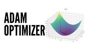
Adam (Adaptive Moment Estimation) is the most popular optimizer because it combines momentum and adaptive learning rates.

🔹 Adam Update Rule:mt=β1∗mt−1+(1−β1)∗∇L(w)vt=β2∗vt−1+(1−β2)∗(∇L(w))2m_t = β_1 * m_{t-1} + (1 – β_1) * ∇L(w) v_t = β_2 * v_{t-1} + (1 – β_2) * (∇L(w))^2 mt​=β1​∗mt−1​+(1−β1​)∗∇L(w)vt​=β2​∗vt−1​+(1−β2​)∗(∇L(w))2

where:

• m_t = first moment estimate (momentum).
• v_t = second moment estimate (variance correction).

🚀 Example: Deep Learning for Self-Driving Cars ✔ SGD struggles with large parameter spaces.
✔ Adam efficiently finds optimal weights, speeding up training.

✅ Best Practice:
✔ Use Adam with default parameters (β1 = 0.9, β2 = 0.999).
✔ Works best for most deep learning models.

---

7. Choosing the Best Optimizer for Your Task

Use Case	Recommended Optimizer
Image Classification (CNNs)	Adam / SGD with momentum
Text Processing (Transformers)	Adam
Recurrent Networks (RNNs, LSTMs)	RMSProp
Sparse Data (NLP, Recommenders)	Adagrad

🚀 Example:
For fine-tuning BERT, Adam is preferred over SGD due to its ability to handle large parameter spaces.

✅ General Rule:
✔ Use Adam for most deep learning tasks.
✔ Use RMSProp for recurrent models.
✔ Use SGD+Momentum for vision tasks.

---

8. Conclusion

Optimization is crucial for efficient deep learning training. The right algorithm can speed up convergence, improve accuracy, and prevent overfitting.

✅ Key Takeaways

✔ Gradient Descent is the foundation of optimization.
✔ Momentum helps escape saddle points and local minima.
✔ Adam is the most widely used adaptive optimizer.
✔ Mini-Batch SGD balances speed and accuracy.
✔ Choosing the right optimizer improves model performance significantly.

💡 Which optimizer do you use for deep learning? Let’s discuss in the comments! 🚀

---

Would you like a Python tutorial comparing Adam, RMSProp, and SGD on a real dataset? 😊