the Difference Between Policy Iteration and Value Iteration in Reinforcement Learning
http://the Difference Between Policy Iteration and Value Iteration in Reinforcement Lea
In reinforcement learning, Policy Iteration and Value Iteration are two fundamental algorithms used to solve Markov Decision Processes (MDPs). These algorithms aim to determine an optimal policy—a mapping from states to actions—that maximizes the expected cumulative reward over time.
This blog dives deep into the concepts of Policy Iteration and Value Iteration, comparing their methods, convergence, and practical use cases, along with detailed explanations. If you’re new to reinforcement learning or need to solidify your understanding, this blog will provide clarity.
What Are Policy Iteration and Value Iteration?
Both Policy Iteration and Value Iteration are dynamic programming approaches for solving MDPs. Let’s explore their definitions and methodologies.
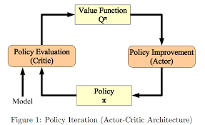
1. Policy Iteration
Policy Iteration consists of two main steps that alternate until convergence:
- Policy Evaluation: Calculate the value function Vπ(s)V^\pi(s) for a fixed policy π\pi. This involves solving the Bellman equation for the given policy.
- Policy Improvement: Update the policy by acting greedily with respect to the current value function.
The process repeats until the policy stops changing, indicating convergence to the optimal policy π∗\pi^*.
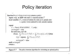
Steps of Policy Iteration:
- Initialize a random policy π0\pi_0.
- Repeat until convergence:
- Evaluate Vπ(s)V^\pi(s) for all states under the current π\pi.
- Improve π\pi by choosing actions that maximize Vπ(s)V^\pi(s).
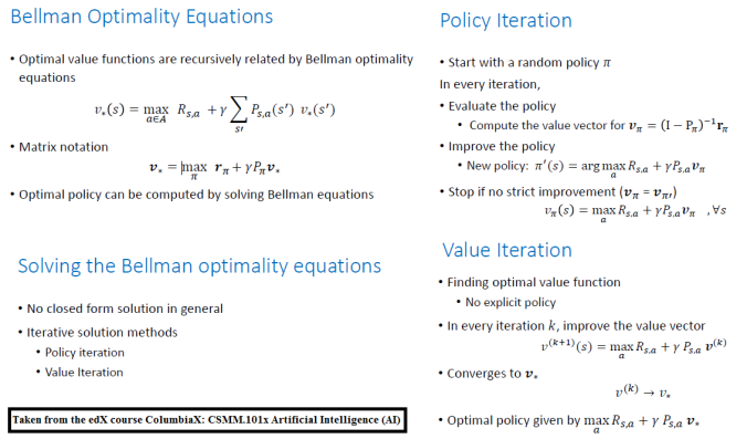
2. Value Iteration
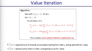
Value Iteration combines policy evaluation and improvement into a single step. Instead of explicitly evaluating the value function for a given policy, it updates the value function iteratively using the Bellman Optimality Equation: Vk+1(s)=maxa∑s′P(s′∣s,a)[R(s,a,s′)+γVk(s′)]V_{k+1}(s) = \max_a \sum_{s’} P(s’|s, a) [R(s, a, s’) + \gamma V_k(s’)]
Where:
- P(s′∣s,a)P(s’|s, a) is the transition probability from state ss to s′s’ under action aa.
- R(s,a,s′)R(s, a, s’) is the reward for transitioning from ss to s′s’.
- γ\gamma is the discount factor.
Steps of Value Iteration:
- Initialize V(s)V(s) arbitrarily for all states.
- Repeat until convergence:
- Update V(s)V(s) using the Bellman Optimality Equation.
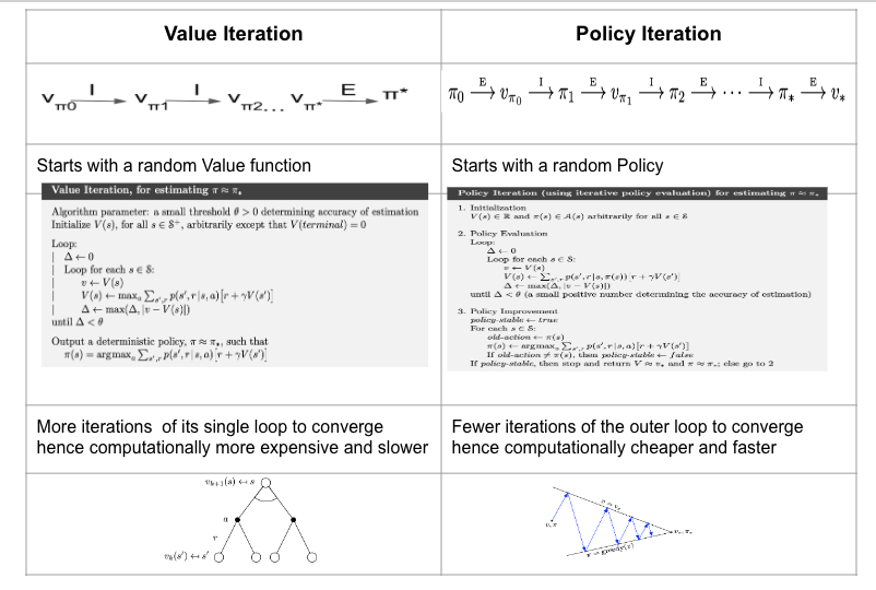
Key Differences Between Policy Iteration and Value Iteration
| Feature | Policy Iteration | Value Iteration |
|---|---|---|
| Approach | Alternates between policy evaluation and improvement. | Iteratively updates the value function directly. |
| Intermediate Steps | Requires solving linear equations for policy evaluation. | Does not require solving linear equations. |
| Convergence | Typically converges in fewer iterations. | Requires more iterations but is computationally simpler. |
| Memory Usage | Requires more memory for policy evaluation. | Requires less memory as it skips explicit policy evaluation. |
| Ease of Implementation | Slightly more complex to implement. | Relatively straightforward to implement. |
Convergence Speed: Which Is Faster?
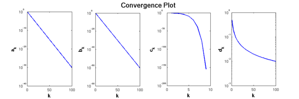
- Policy Iteration tends to converge in fewer iterations because it explicitly evaluates the policy at each step.
- Value Iteration, while requiring more iterations, involves simpler computations per iteration, making it computationally efficient for large state spaces.
In practice:
- Use Policy Iteration when the state space is small or medium, as it provides quicker convergence.
- Use Value Iteration for large state spaces where memory and computational simplicity are critical.
Code Implementation of Policy Iteration and Value Iteration
Below, we provide Python implementations of both algorithms. Each section includes code snippets and explanations, converted to HTML format for easy copying.
Policy Iteration Code
<pre>
<code>
import numpy as np

# Define MDP parameters
states = [0, 1, 2]
actions = [0, 1]
transition_probabilities = {
    (0, 0): [(1.0, 1)],
    (0, 1): [(1.0, 2)],
    (1, 0): [(1.0, 0)],
    (1, 1): [(1.0, 2)],
    (2, 0): [(1.0, 1)],
    (2, 1): [(1.0, 0)],
}
rewards = {
    (0, 0): 0, (0, 1): 10,
    (1, 0): -1, (1, 1): 10,
    (2, 0): 1, (2, 1): -10,
}
gamma = 0.9  # Discount factor

def policy_iteration(states, actions, transition_probabilities, rewards, gamma):
    # Initialize random policy
    policy = {s: np.random.choice(actions) for s in states}
    value_function = {s: 0 for s in states}

    def policy_evaluation(policy, value_function):
        while True:
            delta = 0
            for s in states:
                action = policy[s]
                value = sum([p * (r + gamma * value_function[s_next])
                             for p, s_next in transition_probabilities[(s, action)]])
                delta = max(delta, abs(value_function[s] - value))
                value_function[s] = value
            if delta < 1e-3:
                break

    def policy_improvement(policy, value_function):
        stable = True
        for s in states:
            old_action = policy[s]
            policy[s] = max(actions, key=lambda a: sum(
                [p * (r + gamma * value_function[s_next])
                 for p, s_next in transition_probabilities[(s, a)]]))
            if old_action != policy[s]:
                stable = False
        return stable

    while True:
        policy_evaluation(policy, value_function)
        if policy_improvement(policy, value_function):
            break

    return policy, value_function

optimal_policy, optimal_values = policy_iteration(states, actions, transition_probabilities, rewards, gamma)
print("Optimal Policy:", optimal_policy)
print("Optimal Values:", optimal_values)
</code>
</pre>
Value Iteration Code
<pre>
<code>
def value_iteration(states, actions, transition_probabilities, rewards, gamma):
    value_function = {s: 0 for s in states}

    while True:
        delta = 0
        for s in states:
            max_value = max([
                sum([p * (r + gamma * value_function[s_next])
                     for p, s_next in transition_probabilities[(s, a)]])
                for a in actions])
            delta = max(delta, abs(value_function[s] - max_value))
            value_function[s] = max_value
        if delta < 1e-3:
            break

    policy = {s: max(actions, key=lambda a: sum(
        [p * (r + gamma * value_function[s_next])
         for p, s_next in transition_probabilities[(s, a)]])) for s in states}

    return policy, value_function

optimal_policy, optimal_values = value_iteration(states, actions, transition_probabilities, rewards, gamma)
print("Optimal Policy:", optimal_policy)
print("Optimal Values:", optimal_values)
</code>
</pre>
Practical Use Cases
- Policy Iteration:
- Suitable for smaller MDPs with well-defined transition probabilities.
- Used in applications like robot navigation or inventory management.
- Value Iteration:
- Preferred for large-scale MDPs, such as traffic signal optimization or complex games like chess.
Conclusion
Policy Iteration and Value Iteration are powerful tools for solving MDPs. While Policy Iteration converges faster in terms of iterations, Value Iteration is computationally efficient per iteration. Selecting the right algorithm depends on the size and complexity of the problem at hand.
By understanding the nuances of these algorithms, you can confidently choose the best approach for your reinforcement learning tasks.
Feel free to use the provided code examples as starting points for your projects, and remember to adjust parameters based on your specific needs!